Chapter 6 JointAI: Joint Analysis and Imputation of Incomplete Data in R
This chapter is based on
Nicole S. Erler, Dimitris Rizopoulos and Emmanuel M. E. H. Lesaffre. JointAI: Joint Analysis and Imputation of Incomplete Data in R. (Manuscript in preparation)
Abstract
Missing data occur in many types of studies and typically complicate the analysis. Multiple imputation, either using joint modelling or the more flexible full conditional specification approach, is popular and works well in standard settings. However, in settings involving non-linear associations or interactions, incompatibility of the imputation model with the analysis model is an issue often resulting in bias. Similarly, complex outcomes such as longitudinal or survival outcomes cannot be adequately handled by standard implementations.
In this chapter, we introduce the R package JointAI, which utilizes the Bayesian framework to perform simultaneous analysis and imputation in regression models with incomplete covariates. Using a fully Bayesian joint modelling approach it overcomes the issue of uncongeniality while retaining the attractive flexibility of fully conditional specification multiple imputation by specifying the joint distribution of analysis and imputation models as a sequence of univariate models that can be adapted to the type of variable. JointAI provides functions for Bayesian inference with generalized linear and generalized linear mixed models as well as survival models, that take arguments analogous to their corresponding and well known complete data versions from base R and other packages. Usage and features of JointAI are described and illustrated using various examples and the theoretical background is outlined.
6.1 Introduction
Missing data are a challenge common to the analysis of data from virtually all kinds of studies. Especially when many variables are measured, as in big cohort studies, or when data are obtained retrospectively, e.g., from registries, proportions of missing values up to 50% are not uncommon in some variables.
Multiple imputation, which is often considered the gold standard to handle incomplete data, has its origin in the 1970s and was primarily developed for survey data (Rubin 1987, 2004). One of its first implementations in R (R Core Team 2018) is the package norm (Novo and Schafer 2010), which performs multiple imputation under the joint modelling framework using a multivariate normal distribution (Schafer 1997). Nowadays, multiple imputation using a fully conditional specification (FCS), also called multiple imputation using chained equations (MICE), and its seminal implementation in the R package mice (Van Buuren and Groothuis-Oudshoorn 2011; Van Buuren 2012), is more frequently used.
Datasets have gotten more complex compared to the survey data multiple imputation was developed for. Therefore, more sophisticated methods that can adequately handle the features of modern data and comply with the assumptions made in its analysis are required. Modern studies do not only record univariate outcomes, measured in cross-sectional settings, but outcomes that consist of two or more measurements, such as repeatedly measured or survival outcomes. Furthermore, non-linear effects, introduced by functions of covariates, such as transformations, polynomials or splines, or interactions between variables are considered in the analysis and hence need to be taken into account during imputation.
Standard multiple imputation, either using FCS or a joint modelling approach, e.g., under a multivariate normal distribution, assumes linear associations between all variables. Moreover, FCS requires the outcome to be explicitly specified in each of the linear predictors of the full conditional distributions. In settings where the outcome is more complex than just univariate, this is not straightforward and not generally possible without information loss, leading to misspecified imputation models.
Some extensions of standard multiple imputation have been developed and are implemented in R packages and other software, but the larger part of software for imputation is restricted to standard settings such as cross-sectional survey data. R packages that offer extensions frequently focus on particular settings and researchers need to be familiar with a number of different packages, which often require input and specifications in very different forms. Moreover, most R packages dealing with incomplete data implement multiple imputation, i.e., create multiple imputed datasets, which are then analysed in a second step, followed by pooling of the results.
The R package JointAI (Erler 2019), which is presented in this chapter, follows a different, fully Bayesian approach. It provides a unified framework for both simple and more complex models, using a consistent specification most users will be familiar with from commonly used (base) R functions. By modelling the analysis model of interest jointly with the incomplete covariates, analysis and imputation can be performed simultaneously while assuring compatibility between all sub-models (Erler et al. 2016, 2019). In this joint modelling approach, the added uncertainty due to the missing values is automatically taken into account in the posterior distribution of the parameters of interest, and no pooling of results from repeated analyses is necessary. The joint distribution is specified in a convenient way, using a sequence of conditional distributions that can be specified flexibly according to each type of variable. Since the analysis model of interest defines the first distribution in the sequence, the outcome is included in the joint distribution without the need for it to enter the linear predictor of any of the other models. Moreover, non-linear associations that are part of the analysis model are automatically taken into account for the imputation of missing values. This directly enables our approach to handle complicated models, with complex outcomes and flexible linear predictors.
In the following, we introduce the R package JointAI, which performs joint analysis and imputation of regression models with incomplete covariates under the Missing At Random assumption (Rubin 1976), and explain how data with incomplete covariate information can be analysed and imputed with it. The package is available for download at the Comprehensive R Archive Network (CRAN) under https://CRAN.R-project.org/package=JointAI. Section 6.2 briefly describes the theoretical background. An outline of the general structure of JointAI is given in Section 6.3, followed by an introduction to example datasets that are used throughout this chapter, in Section 6.4. Details about model specification, settings controlling the Markov Chain Monte Carlo sampling, and summary, plotting and other functions that can be applied after fitting the model are given in Sections 6.5 through 6.7. We conclude the paper with an outlook of planned extensions and discuss the limitations that are introduced by the assumptions made in the sequential imputation approach.
6.2 Theoretical Background
Consider the general setting of a regression model where interest lies in a set of parameters \(\boldsymbol\theta\) that describe the association between a univariate outcome \(\mathbf y\) and a set of covariates \(\mathbf X = (\mathbf x_1, \ldots, \mathbf x_p)\). In the Bayesian framework, inference over \(\boldsymbol\theta\) is obtained by estimation of the posterior distribution of \(\boldsymbol\theta\), which is proportional to the product of the likelihood of the data \((\mathbf y, \mathbf X)\) and the prior distribution of \(\boldsymbol\theta\), \[ p(\boldsymbol\theta\mid \mathbf y, \mathbf X) \propto p(\mathbf y, \mathbf X \mid \boldsymbol\theta)\,p(\boldsymbol\theta).\]
When some of the covariates are incomplete, \(\mathbf X\) consists of two parts, the completely observed variables \(\mathbf X_{obs}\) and those variables that are incomplete, \(\mathbf X_{mis}\). If \(\mathbf y\) had missing values (and this missingness was ignorable), the only necessary change in the formulas below would be to replace \(\mathbf y\) by \(\mathbf y_{mis}\). We will, therefore, without loss of generality, consider \(\mathbf y\) to be completely observed.
The likelihood of the complete data, i.e., observed and unobserved, can be factorized in the following convenient way: \[p(\mathbf y, \mathbf X_{obs}, \mathbf X_{mis} \mid \boldsymbol\theta) = p(\mathbf y \mid \mathbf X_{obs}, \mathbf X_{mis}, \boldsymbol\theta_{y\mid x})\, p(\mathbf X_{mis} \mid \mathbf X_{obs}, \boldsymbol\theta_x), \] where the first factor constitutes the analysis model of interest, described by a vector of parameters \(\boldsymbol\theta_{y\mid x}\), and the second factor is the joint distribution of the incomplete variables, i.e., the imputation part of the model, described by parameters \(\boldsymbol\theta_x\), and \(\boldsymbol\theta = (\boldsymbol\theta_{y\mid x}^\top, \boldsymbol\theta_x^\top)^\top\).
Explicitly specifying the joint distribution of all data is one of the major advantages of the Bayesian approach, since this facilitates the use of all available information of the outcome in the imputation of the incomplete covariates (Erler et al. 2016), which becomes especially relevant for more complex outcomes such as repeatedly measured variables (see Section 6.2.2).
In complex models, the posterior distribution can usually not be analytically derived but Markov Chain Monte Carlo (MCMC) methods are used to obtain samples from the posterior distribution. The MCMC sampling in JointAI is done using Gibbs sampling, which iteratively samples from the full conditional distributions of the unknown parameters and missing values.
In the following sections, we describe each of the three parts of the model, the analysis model, the imputation part and the prior distributions, in detail.
6.2.1 Analysis Model
The analysis model of interest is described by the probability density function \(p(\mathbf y \mid \mathbf X, \boldsymbol\theta_{y\mid x})\). The R package JointAI can currently handle analysis models that are either generalized linear regression models (GLM), (generalized) linear mixed models (GLMM), cumulative logit (mixed) models, parametric (Weibull) survival models or Cox proportional hazards models.
For a GLM, the probability density function is chosen from the exponential family and the model has the linear predictor \[g(E(y_i\mid \mathbf X, \boldsymbol\theta_{y\mid x})) = \mathbf x_i^\top\boldsymbol\beta,\] where \(g(\cdot)\) is a link function, \(y_i\) the value of the outcome variable for subject \(i\), and \(\mathbf x_i\) is the row of \(\mathbf X\) that contains the covariate information for \(i\).
For a GLMM the linear predictor is of the form \[g(E(y_{ij}\mid \mathbf X, \mathbf b_i, \boldsymbol\theta_{y\mid x})) = \mathbf x_{ij}^\top\boldsymbol\beta + z_{ij}^\top\mathbf b_i,\] where \(y_{ij}\) is the \(j\)-th outcome of subject \(i\), \(\mathbf x_{ij}\) is the corresponding vector of covariate values, \(\mathbf b_i\) a vector of random effects pertaining to subject \(i\), and \(\mathbf z_{ij}\) the row of the design matrix of the random effects, \(\mathbf Z\), that corresponds to the \(j\)-th measurement of subject \(i\). \(\mathbf Z\) typically contains a subset of the variables in \(\mathbf X\), and \(\mathbf b_i\) follows a normal distribution with mean zero and covariance matrix \(\mathbf D\).
In both cases the parameter vector \(\boldsymbol\theta_{y\mid x}\) contains the regression coefficients \(\boldsymbol\beta\), and potentially additional variance parameters (e.g., for linear (mixed) models), for which prior distributions will be specified in Section 6.2.3.
Cumulative logit mixed models are of the form \[\begin{eqnarray*} y_{ij} &\sim& \text{Multinom}(\pi_{ij,1}, \ldots, \pi_{ij,K}),\\[2ex] \pi_{ij,1} &=& P(y_{ij} \leq 1),\\ \pi_{ij,k} &=& P(y_{ij} \leq k) - P(y_{ij} \leq k-1), \quad k \in 2, \ldots, K-1,\\ \pi_{ij,K} &=& 1 - \sum_{k = 1}^{K-1}\pi_{ij,k},\\[2ex] \text{logit}(P(y_{ij} \leq k)) &=& \gamma_k + \eta_{ij}, \quad k \in 1,\ldots,K,\\ \eta_{ij} &=& x_{ij}^\top\boldsymbol\beta + z_{ij}^\top\mathbf b_i,\\[2ex] \gamma_1,\delta_1,\ldots,\delta_{K-1} &\overset{iid}{\sim}& N(\mu_\gamma, \sigma_\gamma^2),\\ \gamma_k &\sim& \gamma_{k-1} + \exp(\delta_{k-1}),\quad k = 2,\ldots,K, \end{eqnarray*}\] where \(\pi_{ij,k} = P(y_{ij} = k)\) and \(\text{logit}(x) = \log\left(\frac{x}{1-x}\right)\). A cumulative logit regression model for a univariate outcome \(y_i\) can be obtained by dropping the index \(j\) and omitting \(z_{ij}^\top\mathbf b_i\). In cumulative logit (mixed) models, the design matrix \(\mathbf X\) does not contain an intercept, since outcome category specific intercepts \(\gamma_1,\ldots, \gamma_K\) are specified. Here, the parameter vector \(\boldsymbol \theta_{y\mid x}\) includes the regression coefficients \(\boldsymbol\beta\), and the first intercept \(\gamma_1\) and increments \(\delta_1, \ldots, \delta_{K-1}\).
Survival data are typically characterized by the observed event or censoring times, \(T_i\), and the event indicator, \(D_i\), which is equal to one if the event was observed and zero otherwise. JointAI provides two types of models to analyse right censored survival data, a parametric model assuming a Weibull distribution for the true (but partially unobserved) survival times \(T^*\), and a semi-parametric Cox proportional hazards model.
The parametric survival model is implemented as \[\begin{eqnarray*} T_i^* &\sim& \text{Weibull}(1, r_i, s),\\ D_i &\sim& \unicode{x1D7D9}(T_i^* \geq C_i),\\ \log(r_j) &=& - \mathbf x_i^\top\boldsymbol\beta,\\ s &\sim& \text{Exp}(0.01), \end{eqnarray*}\] where \(\unicode{x1D7D9}\;\) is the indicator function which is one if \(T_i^* \geq C_i\), and zero otherwise.
For the Cox proportional hazards model, following Lunn et al. (2012), a counting process representation is implemented, where the baseline hazard is assumed to be piecewise constant and changes only at observed event times. Let \(\{N_i(t), t \geq 0\}\) be an event counting process for individual \(i\), where \(N_i(t) = 0\) until the individual experiences an event and increases by one at the time of the event. \(dN_i(t)\) then denotes the change in \(N_i(t)\) in the interval \([t, t+dt)\), where \(dt\) is the length of that interval, and can be modelled as a Poisson random variable with time-varying intensity \(\lambda_i(t)\). This intensity depends on covariates \(\mathbf x_i\), the baseline hazard \(\lambda_0(t)\), and the risk set indicator \(R_i(t)\), which is equal to one if, at time \(t\), subject \(i\) is at risk for an event, and zero otherwise. \[\begin{eqnarray*} dN(t)_i &\sim& \text{Poisson}(\lambda_i(t)),\quad t \in 0,\ldots, T\\ \lambda_i(t) &=& \exp(\mathbf x_i^\top\boldsymbol\beta) \; \lambda_0(t) \; R_i(t)\\ \lambda_0(t) &\sim& \text{Gamma}(c\lambda_0(t)^*, c) \end{eqnarray*}\] where \(\lambda_0(t)^*\) is a prior guess of the failure rate at time \(t\), and \(c\) represents the confidence about that prior guess.
6.2.2 Imputation Part
A convenient way to specify the joint distribution of the incomplete covariates \(\mathbf X_{mis} = (\mathbf x_{mis_1}, \ldots, \mathbf x_{mis_q})\) is to use a sequence of conditional univariate distributions (Erler et al. 2016; Ibrahim, Chen, and Lipsitz 2002) \(\boldsymbol\theta_{x} = (\boldsymbol\theta_{x_1}^\top, \ldots, \boldsymbol\theta_{x_q}^\top)^\top\).
Each of the conditional distributions is a member of the exponential family, extended with distributions for ordinal categorical variables, and chosen according to the type of the respective variable. Its linear predictor is \[ g_\ell\left\{E\left(x_{i,mis_\ell} \mid \mathbf x_{i,obs}, \mathbf x_{i, mis_{<\ell}}, \boldsymbol\theta_{x_\ell}\right) \right\} = (\mathbf x_{i, obs}^\top, x_{i, mis_1}, \ldots, x_{i, mis_{\ell-1}}) \boldsymbol\alpha_{\ell}, \] for \(\ell=1,\ldots,q\), where \(\mathbf x_{i,mis_{<\ell}} = (x_{i,mis_1}, \ldots, x_{i,mis_{\ell-1}})^\top\).
Factorization of the joint distribution of the covariates in such a sequence yields a straightforward specification of the joint distribution, even when the covariates are of mixed type.
Missing values in the covariates are sampled from their full conditional distributions that can be derived from the full joint distribution of outcome and covariates.
When, for instance, the analysis model is a GLM, the full conditional distribution of an incomplete covariate \(x_{i, mis_{\ell}}\) can be written as \[\begin{eqnarray} p(x_{i, mis_{\ell}} \mid \mathbf y_i, \mathbf x_{i,obs}, \mathbf x_{i,mis_{-\ell}}, \boldsymbol\theta) & \propto& p \left(y_i \mid \mathbf x_{i, obs}, \mathbf x_{i, mis}, \boldsymbol\theta_{y\mid x} \right)\, p(\mathbf x_{i, mis}\mid \mathbf x_{i, obs}, \boldsymbol\theta_{x})\\ & & p(\boldsymbol\theta_{y\mid x})\, p(\boldsymbol\theta_{x})\\\nonumber &\propto& p\left(y_i \mid \mathbf x_{i, obs}, \mathbf x_{i, mis}, \boldsymbol\theta_{y\mid x} \right)\, p(x_{i, mis_\ell} \mid \mathbf x_{i, obs}, \mathbf x_{i, mis_{<\ell}}, \boldsymbol\theta_{x_\ell})\\ & &\left\{\prod_{k=\ell+1}^q p(x_{i,mis_k}\mid \mathbf x_{i, obs}, \mathbf x_{i, mis_{<k}}, \boldsymbol\theta_{x_k}) \right\}\, p(\boldsymbol\theta_{y\mid x}) p(\boldsymbol\theta_{x_\ell})\\ & & \prod_{k=\ell+1}^p \, p(\boldsymbol\theta_{x_k}),\tag{6.2} \end{eqnarray}\] where \(\boldsymbol\theta_{x_{\ell}}\) is the vector of parameters describing the model for the \(\ell\)-th covariate, and contains the vector of regression coefficients and potentially additional (variance) parameters. The product of distributions enclosed by curly brackets represents the distributions of those covariates that have \(x_{mis_\ell}\) as a predictive variable in the specification of the sequence in (6.1).
Even though (6.2) describes the actual imputation model, i.e., the distribution the imputed values for \(x_{i, mis_{\ell}}\) are sampled from, we will use the term “imputation model” for the conditional distribution of \(x_{i, mis_{\ell}}\) from (6.1), since the latter is the distribution that is explicitly specified by the user and, hence, of more relevance when using JointAI.
Imputation with Longitudinal Outcomes
Factorizing the joint distribution into the analysis model and imputation part allows a straightforward extension to settings with more complex outcomes, such as repeatedly measured outcomes. In the case where the analysis model is a GLMM, the conditional distribution of the outcome in (6.2), \(p(y_i \mid \mathbf x_{i, obs}, \mathbf x_{i, mis}, \boldsymbol\theta_{y\mid x})\), has to be replaced by \(\mathbf y\) does not appear in any of the other terms in (6.2), and (6.3) can be chosen to be a model that is appropriate for the outcome at hand, the thereby specified full conditional distribution of \(x_{i, mis_\ell}\) allows us to draw valid imputations that use all available information on the outcome.
This is an important difference to standard FCS, where the full conditional distributions used to impute missing values are specified directly, usually as regression models, and require the outcome to be explicitly included in the linear predictor of the imputation model. In settings with complex outcomes, it is not clear how this should be done, and simplifications may lead to biased results (Erler et al. 2016). The joint model specification utilized in JointAI overcomes this difficulty.
When some of the covariates are time-varying, it is convenient to specify models for these variables at the beginning of the sequence of covariate models, so that models for longitudinal variables have other longitudinal and baseline covariates in their linear predictor, but longitudinal covariates do not enter the predictors of baseline covariates.
Note that whenever there are incomplete baseline covariates it is necessary to specify models for all longitudinal variables, even completely observed ones, while models for completely observed baseline covariates can be omitted. This becomes clear when we extend the factorized joint distribution from above with completely and incompletely observed covariates \(s_{obs}\) and \(s_{mis}\): \[\begin{multline*} p(y_{ij} \mid \mathbf s_{ij, obs}, \mathbf s_{ij, mis}, \mathbf x_{i, obs}, \mathbf x_{i, mis}, \boldsymbol\theta_{y\mid x})\, p(\mathbf s_{ij, mis}\mid \mathbf s_{ij, obs}, \mathbf x_{i, obs}, \mathbf x_{i, mis}, \boldsymbol\theta_{s_{mis}})\\ p(\mathbf s_{ij, obs}\mid \mathbf x_{i, obs}, \mathbf x_{i, mis}, \boldsymbol\theta_{s_{obs}})\, p(\mathbf x_{i, mis}\mid \mathbf x_{i, obs}, \boldsymbol\theta_{x_{mis}})\, p(\mathbf x_{i, obs} \mid \boldsymbol\theta_{x_{obs}})\\ p(\boldsymbol\theta_{y\mid x})\, p(\boldsymbol\theta_{s_{mis}}) \, p(\boldsymbol\theta_{s_{obs}})\, p(\boldsymbol\theta_{x_{mis}}) \, p(\boldsymbol\theta_{x_{obs}}) \end{multline*}\] Given that the parameter vectors \(\boldsymbol\theta_{x_{obs}}\), \(\boldsymbol\theta_{x_{mis}}\), \(\boldsymbol\theta_{s_{obs}}\) and \(\boldsymbol\theta_{s_{mis}}\) are a priori independent, and \(p(\mathbf x_{i, obs} \mid \boldsymbol\theta_{x_{obs}})\) is independent of both \(\mathbf x_{i,mis}\) and \(\mathbf s_{ij,mis}\), it can be excluded from the model.
Since \(p(\mathbf s_{ij, obs}\mid \mathbf x_{i, obs}, \mathbf x_{i, mis}, \boldsymbol\theta_{s_{obs}})\), however, has \(\mathbf x_{i, mis}\) in its linear predictor and will, hence, be part of the full conditional distribution of \(\mathbf x_{i, mis}\), it cannot be omitted from the model specification.
Non-linear Associations and Interactions
Other settings in which the fully Bayesian approach employed in JointAI has an advantage over standard FCS are settings with interaction terms that involve incomplete covariates, or when the association of the outcome with an incomplete covariate is non-linear. In standard FCS such settings lead to incompatible imputation models (White, Royston, and Wood 2011; Bartlett et al. 2015). This becomes clear when considering the following simple example where the analysis model of interest is the linear regression \(y_i = \beta_0 + \beta_1 x_i + \beta_2 x_i^2 + \varepsilon_i\) and \(x_i\) is imputed using \(x_i = \alpha_0 + \alpha_1 y_i + \tilde\varepsilon_i\). While the analysis model assumes a quadratic relationship, the imputation model assumes a linear association between \(\mathbf x\) and \(\mathbf y\) and a joint distribution with these imputation and analysis models as its full conditional distributions does not exist. Because, in JointAI, the analysis model is a factor in the full conditional distribution that is used to impute \(x_i\), the non-linear association is taken into account. Furthermore, since it is the joint distribution that is specified, and the full conditionals are derived from it, the joint distribution is guaranteed to exist.
6.2.3 Prior Distributions
Prior distributions have to be specified for all (hyper)parameters. A common prior choice for the regression coefficients is the normal distribution with mean zero and large variance. In JointAI variance parameters in models for normally distributed variables are specified as inverse-gamma distributions.
The covariance matrix of the random effects in a mixed model, \(\mathbf D\), is assumed to follow an inverse-Wishart distribution where the degrees of freedom are chosen to be equal to the dimension of the random effects and the scale matrix is diagonal. Since the magnitude of the diagonal elements relates to the variance of the random effects, the choice of suitable values depends on the scale of the variable the random effect is associated with. Therefore, JointAI uses independent gamma hyperpriors for each of the diagonal elements. More details about the default hyperparameters and how to change them are given in Section 6.5.8 and Appendix 6.A.
6.3 Package Structure
The package JointAI has seven main functions, lm_imp(),
glm_imp(), clm_imp(), lme_imp(), glme_imp(), clmm_imp(), survreg_imp()
and coxph_imp(),
that perform regression of continuous and categorical, univariate or multi-level
data as well as right censored survival data.
Model specification is similar to that of standard regression
models in R and is described in detail in Section 6.5.
Based on the specified model formula and other arguments that are provided by the user, JointAI does some pre-processing of the data. It checks which variables are incomplete and/or time-varying, and identifies their measurement level in order to specify appropriate (imputation) models. Interactions and functional forms of variables are detected in the model formula and corresponding design matrices for the various parts of the model are created.
MCMC sampling is performed by the program JAGS (Plummer 2003). The JAGS model, data list, containing all necessary parts of the data, and user-specified settings for the MCMC sampling (further described in Section 6.6) are passed to JAGS via the R package rjags (Plummer 2018).
The above named main functions, from here on abbreviated as *_imp(),
all return an object of class JointAI.
Summary and plotting methods for JointAI objects, as well as functions
to evaluate convergence and precision of the MCMC samples, to predict from
JointAI objects and to export imputed values are discussed in Section 6.7.
Currently, the package works under the assumption of a Missing At Random (MAR) missingness process (Rubin 1976, 1987). When this assumption holds, it is valid to exclude cases with missing values in the outcome in Bayesian inference. Hence, our focus here is on missing covariate values. Nevertheless, JointAI can handle missing values in the outcome; they are implicitly imputed using the specified analysis model.
6.4 Example Data
To illustrate the functionality of JointAI we use three
datasets that are part of this package or the package survival (Therneau 2015; Terry M. Therneau and Patricia M. Grambsch 2000).
The first dataset, the NHANES data, contains data from a
cross-sectional cohort study,
whereas the second dataset (simLong) is a simulated dataset based on a
longitudinal cohort study in toddlers.
The third dataset (lung) contains data on survival of patients with advanced lung cancer.
6.4.1 The NHANES Data
The NHANES data is a subset of observations from the 2011 – 2012 wave of
the National Health and Nutrition Examination Survey (National Center for Health Statistics (NCHS) 2011) and
contains information on 186 men and women
between 20 and 80 years of age.
The variables contained in this dataset are
SBP: systolic blood pressure in mmHg; completegender:malevsfemale; completeage: in years; completerace: 5 unordered categories; completeWC: waist circumference in cm; 1.1% missingalc: alcohol consumption;<1drink per week vs>= 1drink per week; 18.3% missingeduc: educational level;lowvshigh; completecreat: creatinine concentration in mg/dL; 4.5% missingalbu: albumin concentration in g/dL; 4.3% missinguricacid: uric acid concentration in mg/dL; 4.3% missingbili: bilirubin concentration in mg/dL; 4.3% missingoccup: occupational status; 3 unordered categories; 15.1% missingsmoke: smoking status; 3 ordered categories; 3.8% missing
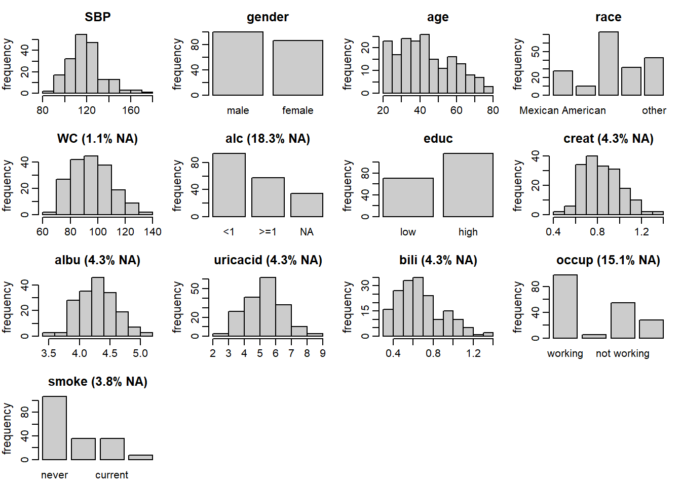
Figure 6.1: Distribution of the variables in the NHANES data (with the
percentage of missing values given for incomplete variables).
Figure 6.1 shows the distributions of all variables
in the NHANES data, together with the proportion of missing
values for incomplete variables, and can be obtained with the function plot_all().
Arguments fill and border allow colours to change,
the number of rows and columns can be adapted using nrow and/or ncol, and
additional arguments can be passed to hist() and barplot() via "...".
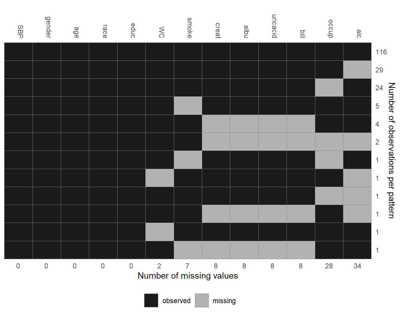
Figure 6.2: Missing data pattern of the NHANES data.
The pattern of missing values in the NHANES data is shown in Figure 6.2.
Each row represents a pattern of missing values, where observed (missing)
values are depicted with dark (light) colour. The frequency with which each of
the patterns is observed is given on the right margin, the number of missing
values in each variable is given underneath the plot. Rows and columns are
ordered by the number of cases per pattern (decreasing) and the number of missing values
(increasing). The first row, for instance, shows that there are 116 complete cases,
the second row that there are 29 cases for which only alc is missing.
Furthermore, it is apparent that creat, albu, uricacid and bili are
always missing together.
Since these variables are all measured in serum this is not surprising.
The plot of the missing data pattern can be obtained with md_pattern().
Again, arguments color and border allow us to change
colours, and arguments such as legend.position, print_xaxis and print_yaxis
permit further customization.
A matrix representation of the missing data pattern can be obtained by setting
pattern = TRUE. There, missing and observed values
are represented with a "0" and "1" respectively.
6.4.2 The simLong Data
The simLong data is a simulated dataset mimicking a longitudinal cohort study
of 200 mother-child pairs. It contains the following
baseline (i.e., not time-varying) covariates
GESTBIR: gestational age at birth in weeks; completeETHN: ethnicity;Europeanvsother; 2.8% missingAGE_M: age of the mother at intake; completeHEIGHT_M: height of the mother in cm; 2.0% missingPARITY: number of times the mother has given birth;0vs>=1; 2.4% missingSMOKE: smoking status of the mother during pregnancy; 3 ordered categories; 12.2% missingEDUC: educational level of the mother; 3 ordered categories; 7.8% missingMARITAL: marital status; 3 unordered categories; 7.0% missingID: subject identifier
and seven longitudinal variables:
time: measurement occasion/visit (by design children should have been measured at 1, 2, 3, 4, 7, 11, 15, 20, 26, 32, 40 and 50 months of age); completeage: child’s age at measurement time in monthshgt: child’s height in cm; 20.0% missingwgt: child’s weight in gram; 8.8% missingbmi: child’s BMI (body mass index) in kg/m2; 21.6% missinghc: child’s head circumference in cm; 23.6% missingsleep: child’s sleeping behaviour; 3 ordered categories; 24.7% missing
Figure 6.3 shows the longitudinal profiles of
hgt, wgt, bmi and hc over age.
All four variables have a non-linear pattern over time.
Distributions of all variables in the simLong data are displayed in
Figure 6.4. Here, arguments use_level and idvar
of the function plot_all() are used to display baseline (level-2) covariates
on the subject level instead of the observation level:
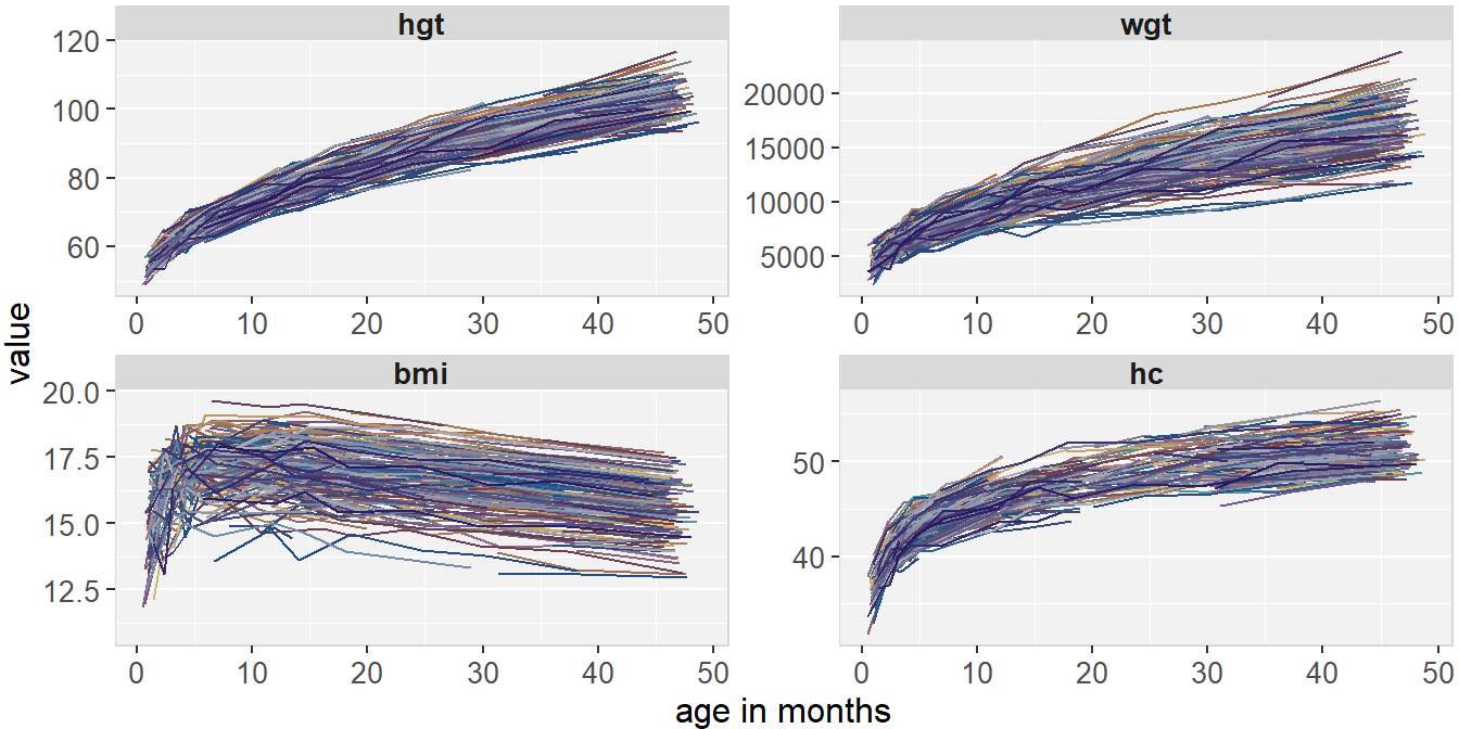
Figure 6.3: Trajectories of height, weight, BMI and head circumference in the simLong data.
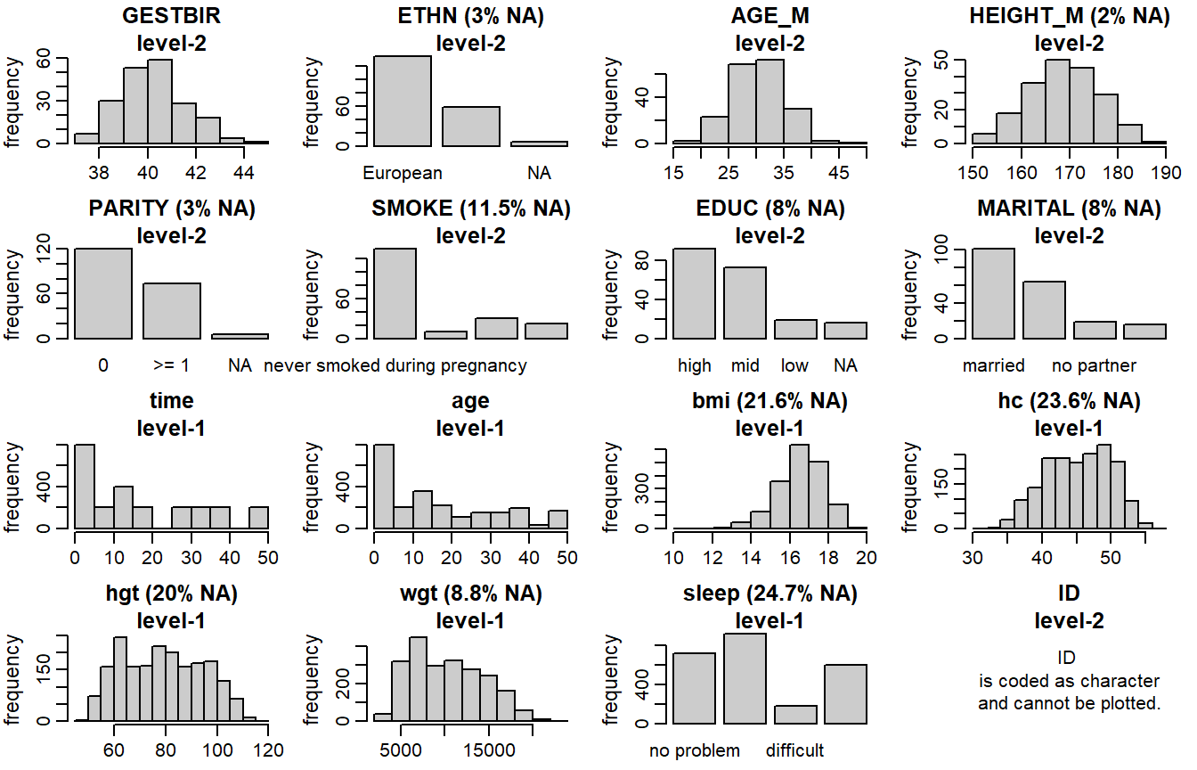
Figure 6.4: Distribution of the variables in the simLong data (with
percentage of missing values given for incomplete variables).
The missing data pattern of the simLong data is shown in Figure 6.5.
For readability, it is plotted separately for baseline (left) and longitudinal
(right) covariates.
Figure 6.5: Missing data pattern.
6.4.3 The lung Data
For demonstration of the use of JointAI for the analysis of survival data,
we use the dataset lung that is included in
the R package survival. It contains data of 228 patients with
advanced lung cancer and includes the following variables:
inst: institution code; completetime: survival time in days; completestatus: event indicator (1: censored,2: dead); completeage: patient’s age in years; completesex: male (1) vs female (2); completeph.ecog: ECOG performance score (describes how the disease impacts the patient’s daily life); scale from0(no impact) to5(dead); 0.4% missingph.karno: Karnofsky performance score as rated by physician (describes the degree of a patient’s impairment by the disease); scale from0(dead) to100(no impairment); 0.4% missingpat.karno: Karnofsky performance score as rated by patient; 1.3% missingmeal.cal: kilocalories consumed at meals; 20.6% missingwt.loss: weight loss over the last six months in kg; 6.1% missing
The distribution of the observed values and the missing data pattern of the lung
data are shown in Figures 6.6 and 6.7.
Figure 6.6: Distribution of the variables in the lung data (with
percentage of missing values given for incomplete variables).
Figure 6.7: Missing data pattern of the lung data.
6.5 Model Specification
The main arguments of the functions
lm_imp(formula, data,
       n.chains = 3, n.adapt = 100, n.iter = 0, thin = 1, ...)

glm_imp(formula, family, data,
        n.chains = 3, n.adapt = 100, n.iter = 0, thin = 1, ...)

clm_imp(formula, data,
        n.chains = 3, n.adapt = 100, n.iter = 0, thin = 1, ...)

lme_imp(fixed, data, random,
        n.chains = 3, n.adapt = 100, n.iter = 0, thin = 1, ...)

glme_imp(fixed, data, random, family,
         n.chains = 3, n.adapt = 100, n.iter = 0, thin = 1, ...)

clmm_imp(fixed, data, random,
         n.chains = 3, n.adapt = 100, n.iter = 0, thin = 1, ...)

survreg_imp(formula, data,
            n.chains = 3, n.adapt = 100, n.iter = 0, thin = 1, ...)

coxph_imp(formula, data,
          n.chains = 3, n.adapt = 100, n.iter = 0, thin = 1, ...)
i.e., formula, data, family, fixed, and random, are used
analogously to the specification in the standard complete data functions
lm() and glm() from package stats, lme() from package nlme (Pinheiro et al. 2018),
and survreg() and coxph() from package survival.
For the description of the remaining arguments see Section 6.6.
The arguments formula (in lm_imp(), glm_imp() and clm_imp()) and fixed
(in lme_imp(), glme_imp() and clmm_imp()) take a standard two-sided formula object,
where an intercept is added automatically.
For the use of the argument random, see Section 6.5.3.
Survival models expect the left hand side of formula to be a survival object
(created with the function Surv() from package survival;
see Section 6.5.4).
The argument family enables the choice of a distribution and link function
from a range of options when using glm_imp() or glme_imp(). The implemented
options are given in Table 6.1.
| family | |
|---|---|
gaussian
|
with links: identity, log
|
binomial
|
with links: logit, probit, log, cloglog
|
Gamma
|
with links: identity, log
|
poisson
|
with links: log, identity
|
6.5.1 Interactions
In JointAI, interactions between any type of variables (observed, incomplete, time-varying) can be handled. When an incomplete variable is involved, the interaction term is re-calculated within each iteration of the MCMC sampling, using the imputed values from the current iteration. Interaction terms involving incomplete variables should hence not be pre-calculated as an additional variable since this would lead to inconsistent imputed values of main effect and interaction term.
Interactions between multiple variables can be specified using parentheses;
for higher lever interactions the "^" operator can be used:
6.5.2 Non-linear Functional Forms
In practice, associations between outcome and covariates do not always meet the standard assumption of linearity. Often, assuming a logarithmic, quadratic or other non-linear effect is more appropriate.
For completely observed covariates, JointAI can handle any common type of
function implemented in R, including splines, e.g., using
ns() or bs() from the package splines.
Since functions involving variables that have missing values need to be
re-calculated in each iteration of the MCMC sampling, currently, only functions
that are available in JAGS can be used for incomplete variables.
Those functions include:
log(),exp()sqrt(), polynomials (usingI())abs()sin(),cos()- algebraic operations involving one or multiple (in)complete variables, as long as the formula can be interpreted by JAGS.
The list of functions implemented in JAGS can be found in the JAGS user manual available at https://sourceforge.net/projects/mcmc-jags/files/Manuals/.
Some examples (that do not necessarily have a meaningful interpretation or good model fit) are:
library("splines")
mod2b <- lm_imp(SBP ~ ns(age, df = 2) + gender + I(bili^2) + I(bili^3),
                data = NHANES)
mod2c <- lm_imp(SBP ~ age + gender + I(creat/albu^2), data = NHANES,
trunc = list(albu = c(1e-5, 1e5)))
# (for explantion of the argument trunc see section below)It is also possible to nest a function in another function.
6.5.2.1 Functions with Restricted Support
When a function of an incomplete variable has restricted support,
e.g., \(\log(x)\) is only defined for \(x > 0\),
or, as in mod2c from above, I(creat/albu^2) can not be calculated for
albu = 0,
the distribution used to impute that variable needs to comply
with these restrictions.
This can either be achieved by truncating the distribution, using the
argument trunc, or by selecting a distribution that meets the restrictions.
Example:
When using a \(\log\) transformation for the covariate bili, we can
use the default imputation method "norm" (a normal distribution) and truncate
it by specifying trunc = list(bili = c(lower, upper)), where lower and
upper are the smallest and largest values allowed:
mod3a <- lm_imp(SBP ~ age + gender + log(bili) + exp(creat),
                trunc = list(bili = c(1e-5, 1e10)), data = NHANES)
Truncation always requires the specification of both limits. Since \(-\text{Inf}\) and \(\text{Inf}\) are not accepted, a value far enough outside the range of the variable (here: \(1e10\)) can be selected for the second boundary of the truncation interval.
Alternatively, we may choose a model for the incomplete variable (using the argument models;
for more details see Section 6.5.5)
that only imputes positive values such as a
log-normal distribution ("lognorm") or a gamma distribution ("gamma"):
Functions Not Available in R
It is possible to use functions that have different names in R and JAGS, or that do exist in JAGS, but not in R, by defining a new function in R that has the name of the function in JAGS.
Example:
In JAGS the inverse logit transformation is defined in the function
ilogit. In base R, there is no function ilogit, but the inverse logit
is available as the distribution function of the logistic distribution plogis().
Thus, we can define the function ilogit() as
and use it in the model formula
A Note on What Happens Inside JointAI
When a function of a complete or incomplete variable is used in the model formula, the main effect of that variable is automatically added as an auxiliary variable (more on auxiliary variables in Section 6.5.6), and only the main effects are used as predictors in the imputation models.
In mod2b, for example, the spline of age is used as predictor for SBP,
but in the imputation model for bili, age enters with a linear effect.
This can be checked using the function
list_models(),
which prints a list of the covariate models used in a JointAI model.
Here, we are only interested in the predictor variables, and, hence,
suppress printing of information on prior distributions, regression coefficients
and other parameters by setting priors, regcoef and otherpars to FALSE:
## Normal imputation model for 'bili'
## * Predictor variables:
##   (Intercept), genderfemale, age
When a function of a variable is specified as an auxiliary variable,
this function is used in the imputation models.
For example, in mod4b, waist circumference (WC)
is not part of the model for SBP, and the quadratic term I(WC^2) is used in
the linear predictor of the imputation model for bili:
mod4b <- lm_imp(SBP ~ age + gender + bili, auxvars = "I(WC^2)",
                data = NHANES)

list_models(mod4b, priors = FALSE, regcoef = FALSE, otherpars = FALSE)
## Normal imputation model for 'WC'
## * Predictor variables:
## (Intercept), age, genderfemale
##
## Normal imputation model for 'bili'
## * Predictor variables:
## (Intercept), age, genderfemale, I(WC^2)Incomplete variables are always imputed on their original scale, i.e.,
in mod2b the variable bili is imputed and the quadratic and cubic versions
are calculated from the imputed values.
Likewise, creat and albu in mod2c
are imputed separately, and I(creat/albu^2) is calculated from the imputed (and
observed) values.
To ensure consistency between variables, functions involving incomplete
variables should be specified as part of the model formula and not be
pre-calculated as separate variables.
6.5.3 Multi-level Structure and Longitudinal Covariates
In multi-level models, additional to the fixed effects structure specified by
the argument fixed, a random effects structure needs to be provided via the
argument random.
Analogous to the specification of the argument random in lme(), it
takes a one-sided formula starting with a "~", and the grouping
variable is separated by "|". A random intercept is added automatically and
only needs to be specified in a random intercept only model.
A few examples:
random = ~1 | id: random intercept only, withidas grouping variablerandom = ~time | id: random intercept and slope for variabletimerandom = ~time + I(time^2) | id: random intercept, slope and quadratic random effect fortimerandom = ~time + x | idrandom intercept, random slope fortimeand random effect for variablex
It is possible to use splines in the random effects structure if there are no missing values in the variables involved, e.g.:
mod5 <- lme_imp(bmi ~ GESTBIR + ETHN + HEIGHT_M + ns(age, df = 2),
                random = ~ ns(age, df = 2) | ID, data = simLong)
Longitudinal (“time-varying”; level-1) covariates can be used in the fixed or random effects and will be imputed if they contain any missing values. Currently only one level of nesting is possible.
6.5.4 Survival Models
JointAI provides two functions to analyse survival data with incomplete
covariates: survreg_imp() and coxph_imp(). Analogous to the complete data
versions of these functions from the package survival, the left-hand side
of the model formula has to be a survival object specified using the function
Surv().
Example:
To analyse the lung data, we can either use a parametric Weibull model
or a Cox proportional hazards model. The survival package needs to be
loaded for the function Surv().
library(survival)
mod6a <- survreg_imp(Surv(time, status) ~ age + sex + ph.karno +
                       meal.cal + wt.loss, data = lung, n.iter = 250)

mod6b <- coxph_imp(Surv(time, status) ~ age + sex + ph.karno + meal.cal +
                     wt.loss, data = lung, n.iter = 250)
Currently only right censored survival data and time-constant covariates can be handled and it is not yet possible to take into account strata, clustering or frailty terms.
6.5.5 Imputation / Covariate Model Types
JointAI automatically selects an (imputation) model for each of the
incomplete baseline (level-2) or longitudinal (level-1) covariates,
based on the class of the variable and the number of levels.
The automatically selected types for baseline covariates are:
norm: linear model (default for continuous variables)logit: binary logistic model (default for factors with two levels)multilogit: multinomial logit model (default for unordered factors with \(>2\) levels)cumlogit: cumulative logit model (default for ordered factors with \(>2\) levels)
The default methods for longitudinal covariates are:
lmm: linear mixed model (default for continuous longitudinal variables)glmm_logit: logistic mixed model (default for longitudinal factors with two levels)clmm: cumulative logit mixed model (default for longitudinal ordered factors with >2 levels)
When a continuous variable has only two different values,
it is automatically converted to a factor and imputed using a logistic model,
unless an imputation model type is specified by the user. Variables of type
logical are automatically converted to binary factors.
The imputation models that are chosen by default may not necessarily be appropriate for the data at hand, especially for continuous variables, which often do not comply with the assumptions of (conditional) normality.
Therefore, the following alternative imputation methods are available for continuous baseline covariates:
lognorm: normal model for the log-transformed variable (right-skewed variables \(>0\))gamma: gamma model with log-link (right-skewed variables \(>0\))beta: beta model with logit-link (continuous variables in \([0, 1]\))
lognorm assumes a (conditional) normal distribution for the natural logarithm
of the variable, but the variable enters the linear predictor of the analysis
model (and possibly other imputation models) on its original scale.
For longitudinal covariates the following alternative model types are available:
glmm_gamma: gamma mixed model with log-link (right-skewed variables \(>0\))glmm_poisson: Poisson mixed model with log-link (count variables)
Specification of Imputation/Covariate Model Types
In models mod3b and mod3c in Section 6.5.2.1 we have already
seen two examples in which the imputation model type was changed using the
argument models, which takes a named vector.
When the vector supplied to models only contains specifications for a subset
of the incomplete and longitudinal covariates, default models
are used for the remaining covariates.
As explained in Section 6.2.2, models for completely observed
longitudinal covariates only need to be specified when any baseline
covariates have missing values.
mod7a <- lm_imp(SBP ~ age + gender + WC + alc + bili + occup + smoke,
                models = c(WC = 'gamma', bili = 'lognorm'),
                data = NHANES, n.iter = 100)

mod7a$models
## WC smoke bili occup alc
## "gamma" "cumlogit" "lognorm" "multilogit" "logit"The function get_models(), which finds and assigns the default imputation
methods, can be called directly.
get_models() has arguments
fixed: the fixed effects formularandom: the random effects formula (if necessary)data: the datasetauxvars: an optional vector of auxiliary variablesno_model: an optional vector of names of covariates for which no model will be specified
mod7b_models <- get_models(bmi ~ GESTBIR + ETHN + HEIGHT_M + SMOKE + hc +
                             MARITAL + ns(age, df = 2),
                           random = ~ ns(age, df = 2) | ID,
                           data = simLong)
mod7b_models
## $models
## HEIGHT_M ETHN MARITAL SMOKE age
## "norm" "logit" "multilogit" "cumlogit" "lmm"
## hc
## "lmm"
##
## $meth
## HEIGHT_M ETHN MARITAL SMOKE hc
## "norm" "logit" "multilogit" "cumlogit" "lmm"get_models() returns a list of two vectors:
models: containing all specified modelsmeth: containing the models for the incomplete variables only
When there is a “time” variable in the model, such as age in our example
(which is the age of the child at the time of the measurement),
it may not be meaningful to specify a model for that variable.
Especially when the “time” variable is pre-specified by the design of the study,
it can usually be assumed to be independent of baseline covariates and a model for it
has no useful interpretation.
The argument no_model (in get_models() and in the main
functions *_imp()) allows for the exclusion of models for such variables
(as long as they are completely observed):
mod7c_models <- get_models(bmi ~ GESTBIR + ETHN + HEIGHT_M + SMOKE + hc +
                             MARITAL + ns(age, df = 2),
                           random = ~ ns(age, df = 2) | ID,
                           data = simLong, no_model = "age")
# mod7c_models
By excluding the model for age we implicitly assume that incomplete baseline
variables are independent of age.
Order of the Sequence of Imputation Models
By default, models for level-1 covariates are specified after models for level-2 covariates, so that the level-2 covariates are used as predictor variables in the models for level-1 covariates but not vice versa. Within the two groups, models are ordered by the number of missing values (decreasing), so that the model for the variable with the most missing values has the most variables in its linear predictor.
6.5.6 Auxiliary Variables
Auxiliary variables are variables that are not part of the analysis model but should be considered as predictor variables in the imputation models because they can inform the imputation of unobserved values.
Good auxiliary variables are (Van Buuren 2012)
- associated with an incomplete variable of interest, or are
- associated with the missingness of that variable and
- do not have too many missing values themselves. Importantly, they should be observed for a large proportion of the cases that have a missing value in the variable to be imputed.
In *_imp(), auxiliary variables can be
specified with the argument auxvars, which is a vector containing the names
of the auxiliary variables.
Example:
We might consider the variables educ and smoke as predictors
for the imputation of occup:
mod8a <- lm_imp(SBP ~ gender + age + occup, auxvars = c('educ', 'smoke'),
                data = NHANES, n.iter = 100)
The variables educ and smoke are not included in the analysis model
(as can be seen when printing the posterior mean of the regression coefficients
of the analysis model with coef()):
##           (Intercept)          genderfemale                   age
##           105.5937694            -5.8192149             0.3781785
## occuplooking for work      occupnot working
##             4.0294291            -0.7349338
They are, however, used as predictors in the imputation for occup and
imputed themselves (if they have missing values):
## Cumulative logit imputation model for 'smoke'
## * Predictor variables:
##   genderfemale, age, educhigh
##
## Multinomial logit imputation model for 'occup'
## * Predictor variables:
##   (Intercept), genderfemale, age, educhigh, smokeformer, smokecurrent
Functions of Variables as Auxiliary Variables
As shown above in mod3e, it is possible to specify functions of
auxiliary variables. In that case, the auxiliary variable is not considered as
a linear effect but as specified by the function.
Note that omitting auxiliary variables from the analysis model implies that the outcome is independent of these variables, conditional on the other variables in the model. If this is not true, the model is misspecified which may lead to biased results (similar to leaving a confounding variable out of a model).
6.5.7 Reference Values for Categorical Covariates
In JointAI, dummy coding is used when categorical variables enter a linear predictor, i.e., a binary variable is created for each category, except the reference category. These binary variables have value one when that category was observed and zero otherwise. Contrary to the behaviour in base R, this coding is also used for ordered factors.
By default, the first category of a categorical variable (ordered or unordered)
is used as reference, however, this may not always allow the desired interpretation
of the regression coefficients. Moreover, when categories are unbalanced, setting
the largest group as reference may result in better mixing of the MCMC chains.
Therefore, JointAI allows specification of the reference category separately
for each variable, via the argument refcats.
Changes in refcats will not impact the imputation of the respective variable,
but change categories for which dummy variables are included in the linear
predictor of the analysis model or other covariate models.
Setting Reference Categories for All Variables
To specify the choice of reference category globally for all variables in the
model, refcats can be set as
refcats = "first"refcats = "last"refcats = "largest"
For example:
Setting Reference Categories for Individual Variables
Alternatively, refcats takes a named vector, in which the reference category
for each variable can be specified either by its number or its name, or one of
the three global types: "first", "last" or "largest".
For variables for which no reference category is specified in the list the
default is used.
mod9b <- lm_imp(SBP ~ gender + age + race + educ + occup + smoke,
                refcats = list(occup = "not working", race = 3,
                               educ = "largest"), data = NHANES)
To facilitate specification of the reference categories, the function
set_refcat()
can be used.
It prints the names of the categorical variables that are selected by
- a specified model formula and/or
- a vector of auxiliary variables, or
- a vector naming covariates,
or all categorical variables in the data if only the argument data is provided,
and asks a number of questions which the user needs to reply to via input of
a number.
##
## How do you want to specify the reference categories?
##
## 1: Use the first category for each variable.
## 2: Use the last category for each variabe.
## 3: Use the largest category for each variable.
## 4: Specify the reference categories individually.
When option 4 is chosen, a choice is given for each categorical variable, for example:
#> The reference category for "race" should be
#>
#> 1: Mexican American
#> 2: Other Hispanic
#> 3: Non-Hispanic White
#> 4: Non-Hispanic Black
#> 5: other
After specification of the reference categories,
the determined specification for the argument refcats is printed:
#> In the JointAI model specify:
#>  refcats = c(gender = 'female', race = 'Non-Hispanic White',
#>              educ = 'low', occup = 'not working', smoke = 'never')
#>
#> or use the output of this function.
set_refcat() also returns a named vector that can be passed to the argument
refcats:
6.5.8 Hyperparameters
In the Bayesian framework, parameters are random variables for which a distribution needs to be specified. These distributions depend on parameters themselves, i.e., on hyperparameters.
The function default_hyperpars() returns a list containing the default
hyperparameters used in a JointAI model (see Appendix 6.A).
To change the hyperparameters in a JointAI model, the list obtained from
default_hyperpars() can be edited and passed to the argument hyperpars
in *_imp().
mu_reg_* and tau_reg_* refer to the mean and precision of the prior distribution
for regression coefficients.
shape_tau_* and rate_tau_* are the shape and rate parameters of a gamma
distribution that is used as prior for precision parameters.
RinvD is the scale matrix in the Wishart prior for the inverse of the random
effects design matrix D, and KinvD is the number of degrees of freedom in that
distribution. shape_diag_RinvD and rate_diag_RinvD are the shape and rate parameters
of the gamma prior of the diagonal elements of RinvD.
In random effects models with only one random effect, a gamma prior is used
instead of the Wishart distribution for the inverse of D.
The hyperparameters mu_reg_surv and tau_reg_surv are used in
survreg_imp() as well as coxph_imp(). For the Cox proportional
hazards model, the hyperparameters c, r and eps refer to
the confidence in the prior guess for the hazard function, failure rate per unit time
(\(\lambda_0(t)^*\) in Section 6.2.1) and time increment
(for numerical stability), respectively.
6.5.9 Scaling
When variables are measured on very different scales this can result in slow convergence and bad mixing. Therefore, JointAI automatically scales continuous variables to have mean zero and standard deviation one. Results (parameters and imputed values) are transformed back to the original scale when the results are printed or imputed values are exported.
In some settings, however, it is not possible to scale continuous variables. This is the case for incomplete variables that enter a linear predictor in a function and variables that are imputed with models that are defined on a subset of the real line (i.e., with a gamma or a beta distribution). Variables that are imputed with a log-normal distribution are scaled, but not centred.
To prevent scaling, the argument scale_vars can be set to FALSE. When
a vector of variable names is supplied to scale_vars, only those variables
are scaled.
By default, only the MCMC samples that are scaled back to the scale of the data
are stored in a JointAI object.
When the argument keep_scaled_mcmc = TRUE, the scaled sample is also kept.
6.5.10 Ridge Regression
Using the argument ridge = TRUE it is possible to impose a ridge penalty
on the parameters of the analysis model, shrinking these parameters towards zero.
This is done by specification of a \(\text{Gamma}(0.01, 0.01)\) prior for the
precision of the regression coefficients \(\beta\) instead of setting it to a
fixed (small) value.
6.6 MCMC Settings
The functions *_imp() have a number of arguments that specify settings for
the MCMC sampling:
n.chains: number of MCMC chainsn.adapt: number of iterations in the adaptive phasen.iter: number of iterations in the sampling phasethin: thinning degreemonitor_params: parameters/nodes to be monitoredseed: optional seed value for reproducibilityinits: initial valuesparallel: whether MCMC chains should be sampled in parallelncores: how many cores are available for parallel sampling
The first four, as well as the following two parameters, are passed directly to functions from the R package rjags:
quiet: should printing of information be suppressed?progress.bar: type of progress bar ("text","gui"or"none")
In the following sections, the arguments listed above are explained in more detail and examples are given.
6.6.1 Number of Chains, Iterations and Samples
Number of Chains
To evaluate convergence of MCMC chains it is helpful to create multiple chains that have different starting values. More information on how to evaluate convergence and the specification of initial values can be found in Sections 6.7.3.1 and 6.6.3 respectively.
The argument n.chains selects the number of chains (by default, n.chains = 3).
For calculating the model summary, multiple chains are merged.
Adaptive Phase
JAGS has an adaptive mode, in which samplers are optimized (for example the
step size is adjusted).
Samples obtained during the adaptive mode do not form a Markov chain and are
discarded.
The argument n.adapt controls the length of this adaptive phase.
The default value for n.adapt is 100, which works well in many of the examples
considered here. Complex models may require longer adaptive phases. If the adaptive
phase is not sufficient for JAGS to optimize the samplers, a warning message will be
printed (see example below).
Sampling Iterations
n.iter specifies the number of iterations in the sampling phase, i.e., the length
of the MCMC chain. How many samples are required to reach convergence and to
have sufficient precision (see also Section 6.7.3.2)
depends on the complexity of data and model, and may
range from as few as 100 to several million.
Thinning
In settings with high autocorrelation, it may take many iterations before a
sample is created that sufficiently
represents the whole range of the posterior distribution.
Processing of such long chains can be slow and cause memory issues.
The parameter thin allows the user to specify if and how much the MCMC chains should
be thinned out before storing them. By default thin = 1 is used,
which corresponds to keeping all values. A value thin = 10 would result in
keeping every 10th value and discarding all other values.
6.6.1.1 Example: Default Settings
Using the default settings n.adapt = 100 and thin = 1, and 100 sampling
iterations, a simple model would be
The relevant part of the model summary (obtained with summary())
shows that the first 100 iterations
(adaptive phase) were discarded, the 100 iterations that follow form the
posterior sample, thinning was set to “1” and there are three chains.
## [...]
## MCMC settings:
## Iterations = 101:200
## Sample size per chain = 100
## Thinning interval = 1
## Number of chains = 3
Example: Insufficient Adaptation Phase
## Warning in rjags::jags.model(file = modelfile, data = data_list, inits
## = inits, : Adaptation incomplete
## NOTE: Stopping adaptation
Specifying n.adapt = 10 results in a warning message. The relevant part of the
model summary from the resulting model is:
## [...]
## Iterations = 11:110
## Sample size per chain = 100
## Thinning interval = 1
## Number of chains = 3
Example: Thinning
Here, iterations 110 until 600 are used in the output, but due to a thinning interval of ten, the resulting MCMC chains contain only 50 samples instead of 500, that is, the samples from iteration 110, 120, 130,
## [...]
## Iterations = 110:600
## Sample size per chain = 50
## Thinning interval = 10
## Number of chains = 3
6.6.2 Parameters to Follow
Since JointAI uses JAGS (Plummer 2003) for performing the MCMC sampling, and JAGS only saves the values of MCMC chains for those nodes which the user has specified should be monitored, this is also the case in JointAI.
For this purpose, the main functions *_imp() have an argument
monitor_params, which takes a named list (or a named vector) with
possible entries given in Table 6.2.
This table contains a number of keywords that refer to (groups of) nodes.
Each of the keywords works as a switch and can be specified as TRUE or FALSE
(with the exception of other).
| name/keyword | what is monitored |
|---|---|
analysis_main
|
betas and sigma_y (and D)
|
betas
|
regression coefficients of the analysis model |
tau_y
|
precision of the residuals from the analysis model |
sigma_y
|
std. deviation of the residuals from the analysis model |
analysis_random
|
ranef, D, invD, RinvD
|
ranef
|
random effects |
D
|
covariance matrix of the random effects |
invD
|
inverse of D
|
RinvD
|
scale matrix in Wishart prior for invD
|
imp_pars
|
alphas, tau_imp, gamma_imp, delta_imp
|
alphas
|
regression coefficients in the imputation models |
tau_imp
|
precision of the residuals from imputation models |
gamma_imp
|
intercepts in ordinal imputation models |
delta_imp
|
increments of ordinal intercepts |
imps
|
imputed values |
other
|
additional parameters |
Parameters of the Analysis Model
The default setting is monitor_params = c(analysis_main = TRUE), i.e.,
only the main parameters of the analysis model are monitored, and
monitoring is switched off for all other parameters.
Main parameters are the regression coefficients of the analysis model
(beta), depending on the model type, the residual standard deviation (sigma_y),
and, for mixed models, the random effects variance-covariance matrix D.
The function parameters() returns the parameters specified to be followed
(also for models where no MCMC sampling was performed, i.e., when n.iter = 0 and
n.adapt = 0). We use it here to demonstrate the effect that different choices
for monitor_params have.
For example:
## [1] "(Intercept)"  "genderfemale" "WC"           "alc>=1"
## [5] "creat"        "sigma_SBP"
Parameters of the Covariate Models and Imputed Values
The parameters of the models for the incomplete variables can be selected with
monitor_params = c(imp_pars = TRUE). This will set monitors for the
regression coefficients (alpha) and other parameters, such as precision
(tau_*) and intercepts and increments (gamma_* and delta_*) in cumulative
logit models.
mod11b <- lm_imp(SBP ~ age + WC + alc + smoke + occup,
                 data = NHANES, n.adapt = 0,
                 monitor_params = c(imp_pars = TRUE,
                                    analysis_main = FALSE))

parameters(mod11b)
## [1] "alpha" "tau_WC" "gamma_smoke" "delta_smoke"To generate (multiple) imputed datasets to be used for further analyses,
the imputed values need to be monitored. This can be achieved by setting
monitor_params = c(imps = TRUE).
mod11c <- lm_imp(SBP ~ age + WC + alc + smoke + occup,
                 data = NHANES, n.adapt = 0,
                 monitor_params = c(imps = TRUE, analysis_main = FALSE))
Extraction of multiple imputed datasets from a JointAI model is described in Section 6.7.6.
Random Effects
For mixed models, analysis_main also includes the random effects variance-covariance
matrix D.
Setting analysis_random = TRUE will switch on monitoring
for the random effects (ranef), random effects variance-covariance matrix (D),
inverse of the random effects variance-covariance matrix (invD) and the diagonal of the
scale matrix of the Wishart-prior of invD (RinvD).
mod11d <- lme_imp(bmi ~ age + EDUC, random = ~age | ID,
                  data = simLong, n.adapt = 0,
                  monitor_params = c(analysis_random = TRUE))

parameters(mod11d)
## [1] "(Intercept)" "EDUCmid" "EDUClow" "age" "sigma_bmi"
## [6] "b" "invD[1,1]" "invD[1,2]" "invD[2,2]" "D[1,1]"
## [11] "D[1,2]" "D[2,2]" "RinvD[1,1]" "RinvD[2,2]"It is possible to select only a subset of the random effects parameters by specifying them directly, e.g.,
mod11e <- lme_imp(bmi ~ age + EDUC, random = ~age | ID,
                  data = simLong, n.adapt = 0,
                  monitor_params = c(analysis_main = TRUE, RinvD = TRUE))

parameters(mod11e)
## [1] "(Intercept)" "EDUCmid" "EDUClow" "age" "sigma_bmi"
## [6] "D[1,1]" "D[1,2]" "D[2,2]" "RinvD[1,1]" "RinvD[2,2]"or by switching unwanted parts of analysis_random off, e.g.,
mod11f <- lme_imp(bmi ~ age + EDUC, random = ~age | ID, data = simLong,
                  n.adapt = 0, monitor_params = c(analysis_main = TRUE,
                                                  analysis_random = TRUE,
                                                  RinvD = FALSE,
                                                  ranef = FALSE))

parameters(mod11f)
## [1] "(Intercept)" "EDUCmid" "EDUClow" "age" "sigma_bmi"
## [6] "invD[1,1]" "invD[1,2]" "invD[2,2]" "D[1,1]" "D[1,2]"
## [11] "D[2,2]"Other Parameters
The element other in monitor_params allows for the specification of one or multiple
additional parameters to be monitored. When other is used with more than one
element, monitor_params has to be a list.
Here, as an example, we monitor the probability of being in the alc>=1 group for
subjects one through three and the expected value of the distribution of creat for
the first subject.
mod11g <- lm_imp(SBP ~ gender + WC + alc + creat, data = NHANES,
                 n.adapt = 0,
                 monitor_params = list(analysis_main = FALSE,
                                       other = c('p_alc[1:3]',
                                                 "mu_creat[1]")))

parameters(mod11g)
## [1] "p_alc[1:3]" "mu_creat[1]"Even though this example may not be particularly meaningful, in cases of convergence issues it can be helpful to be able to monitor any node of the model, not just the ones that are typically of interest.
6.6.3 Initial Values
Initial values are the starting point for the MCMC sampler. Setting good
initial values, i.e., values that are likely under the posterior distribution,
can speed up convergence.
By default, the argument inits = NULL, which means that initial values are
generated automatically by JAGS.
It is also possible to supply initial values directly as a list or as a function.
Initial values can be specified for every unobserved node, that is, parameters and missing values, but it is possible to only specify initial values for a subset of nodes.
When the initial values provided by the user do not have elements named
".RNG.name" or ".RNG.seed", JointAI will add those elements,
which specify the name and seed value of the random number generator used
for each chain.
The argument seed allows the specification of a seed value with which the
starting values of the random number generator, and, hence, the values of the MCMC
sample, can be reproduced.
Initial Values in a List of Lists
A list containing initial values should have the same length as the number of chains, where each element is a named list of initial values. Moreover, initial values should differ between the chains.
For example, to create initial values for the parameter vector beta and
the precision parameter tau_SBP for two chains the following syntax could
be used:
init_list <- lapply(1:2, function(i) {
  list(beta = rnorm(4),
       tau_SBP = rgamma(1, 1, 1))
})

init_list
## [[1]]
## [[1]]$beta
## [1] 0.2995096 0.2123710 0.6478957 0.8952516
##
## [[1]]$tau_SBP
## [1] 1.000624
##
##
## [[2]]
## [[2]]$beta
## [1] 2.2559981 0.9786635 -1.2725176 -0.7251253
##
## [[2]]$tau_SBP
## [1] 0.05501739The user provided lists of initial values are stored in the JointAI object
(together with starting values for the random number generator)
and can be accessed via mod11a$mcmc_settings$inits.
Initial Values as a Function
Initial values can be specified as a function. The function should either take no
arguments or a single argument called chain, and return a named list that
supplies values for one chain.
For example, to create initial values for the parameter vectors beta and alpha:
## $beta
## [1] -1.6045542  0.1872611  1.0167161 -0.4272887
##
## $alpha
## [1] 0.8542140 0.6391477 0.4720952
mod12b <- lm_imp(SBP ~ gender + age + WC, data = NHANES,
inits = inits_fun)
mod12b$mcmc_settings$inits## [[1]]
## [[1]]$beta
## [1] -0.07058338 0.41772091 -1.66236440 1.24957652
##
## [[1]]$alpha
## [1] -0.7204577 0.1424769 -1.0114044
##
## [[1]]$.RNG.name
## [1] "base::Wichmann-Hill"
##
## [[1]]$.RNG.seed
## [1] 77704
##
##
## [[2]]
## [[2]]$beta
## [1] -0.50236788 -0.01997157 1.40425944 1.18807193
##
## [[2]]$alpha
## [1] -0.8065902 -0.9709539 -0.7020397
##
## [[2]]$.RNG.name
## [1] "base::Mersenne-Twister"
##
## [[2]]$.RNG.seed
## [1] 29379
##
##
## [[3]]
## [[3]]$beta
## [1] -0.3516978 -0.9144069 -1.7397631 -0.1083395
##
## [[3]]$alpha
## [1] 0.9067457 -0.4471829 0.1170837
##
## [[3]]$.RNG.name
## [1] "base::Mersenne-Twister"
##
## [[3]]$.RNG.seed
## [1] 83619When a function is supplied, the function is evaluated by JointAI and the
resulting list is stored in the JointAI object.
6.6.3.1 For which Nodes can Initial Values be Specified?
Initial values can be specified for all unobserved stochastic nodes, i.e.,
parameters or unobserved data for which a distribution is specified in the
JAGS model. They have to be supplied in the format of the parameter or unobserved
value in the JAGS model.
To find out which nodes there are in a model and in which form they have to be
specified,
the function coef() from package rjags can be used to obtain a list
with the current values of the MCMC chains (by default the first chain)
from a JAGS model object. This object is contained in a JointAI
object under the name model.
Elements of the initial values should have the same structure as the elements in
this list of current values.
Example:
We are using a longitudinal model and the simLong data in this example.
Here we only show some relevant parts of the output.
mod12c <- lme_imp(bmi ~ time + HEIGHT_M + hc + SMOKE, random = ~ time | ID,
                  no_model = 'time', data = simLong)

# coef(mod12c$model)
RinvD is the scale matrix in the Wishart prior for the inverse of the
random effects variance-covariance matrix D.
In the data that is passed to JAGS (which is stored in the element data_list
in a JointAI object), this matrix is specified as a diagonal matrix,
with unknown diagonal elements:
## $RinvD
##      [,1] [,2]
## [1,]   NA    0
## [2,]    0   NA
These diagonal elements are estimated in the model and have a gamma prior. The corresponding part of the JAGS model is:
## [...]
##   # Priors for the covariance of the random effects
##   for (k in 1:2){
##     RinvD[k, k] ~ dgamma(shape_diag_RinvD, rate_diag_RinvD)
##   }
##   invD[1:2, 1:2] ~ dwish(RinvD[ , ], KinvD)
##   D[1:2, 1:2] <- inverse(invD[ , ])
## [...]
The element RinvD in the initial values has to be a \(2\times2\) matrix,
with positive values on the diagonal and NA as off-diagonal elements,
since these are fixed in the data:
## $RinvD
##            [,1]       [,2]
## [1,] 0.03648925         NA
## [2,]         NA 0.07655993
Lines 82 through 85 of the design matrix of the fixed effects of baseline
covariates, Xc, in the data are:
##       (Intercept)  HEIGHT_M SMOKEsmoked until[...] SMOKEcontin[...]
## 172.1           1 0.1148171                     NA               NA
## 173.1           1        NA                     NA               NA
## 174.1           1 0.5045126                     NA               NA
## 175.1           1 1.8822249                     NA               NA
The matrix Xc in the initial values has the same dimension as Xc in the
data. It has values where there are missing values in Xc in the data,
e.g., Xc[83, 2], and is NA elsewhere:
## $Xc
##        [,1]       [,2] [,3] [,4]
##   [1,]   NA         NA   NA   NA
##
## [...]
##
##  [82,]   NA         NA   NA   NA
##  [83,]   NA  0.8028938   NA   NA
##  [84,]   NA         NA   NA   NA
##
## [...]
There are no initial values specified for the third and fourth column, since
these columns contain the dummy variables corresponding to the categorical
variable SMOKE and are calculated from the corresponding column in the matrix Xcat,
i.e., these are deterministic nodes, not stochastic nodes.
The relevant part of the JAGS model is:
## [...]
##     # ordinal model for SMOKE
##     Xcat[i, 1] ~ dcat(p_SMOKE[i, 1:3])
## [...]
##     Xc[i, 3] <- ifelse(Xcat[i, 1] == 2, 1, 0)
##     Xc[i, 4] <- ifelse(Xcat[i, 1] == 3, 1, 0)
## [...]
Elements that are completely unobserved, like the parameter vectors alpha
and beta, the random effects b or scalar parameters delta_SMOKE and
gamma_SMOKE are entirely specified in the initial values.
6.6.4 Parallel Sampling
To reduce the computational time it is possible to perform sampling of multiple
MCMC chains in parallel. This can be specified by setting
the argument parallel = TRUE. The maximum number of cores to be used can be
set with the argument ncores. By default this is two less than the number of
cores available on the machine, but never more than the number of MCMC chains.
Parallel computation is done using the packages foreach (Microsoft and Weston 2017) and doParallel (Corporation and Weston 2018). Note that it is currently not possible to display a progress bar when using parallel computation.
6.7 After Fitting
Any of the main functions *_imp() will return an object of class JointAI.
It contains the original data (data),
information on the type of model (call, analysis_type, models,
fixed, random, hyperpars, scale_pars)
and MCMC sampling (mcmc_settings),
the JAGS model (model) and MCMC sample (MCMC; if a sample was
generated), the computational time (time)
of the MCMC sampling, and some additional
elements that are used by methods for objects of class JointAI
but are typically not of interest for the user.
In the remaining part of this section, we describe how the results from a
JointAI model can be visualized, summarized and evaluated.
The functions described here use, by default, the full MCMC sample
and show only the parameters of the analysis model.
Arguments start, end and thin are available to select a subset of the MCMC
samples that is used to calculate the summary. The argument subset allows the user to control
for which nodes the summary or visualization is returned
and follows the same logic as
the argument monitor_params in *_imp().
The use of these arguments is further explained in Section 6.7.4.
6.7.1 Visualizing the Posterior Sample
The posterior sample can be visualized by two commonly used plots: a traceplot, showing samples across iterations, and a plot of the empirical density of the posterior sample.
Traceplot
A traceplot shows the sampled values per chain and node throughout
iterations. It allows the visual evaluation of convergence and mixing of the chains
and can be obtained with the function traceplot().
Figure 6.8: Traceplot of mod13a.
When the sampler has converged the chains show one horizontal band, as in
Figure 6.8.
Consequently, when traces show a trend, convergence has not been
reached and more iterations are necessary (e.g., using add_samples()).
Graphical aspects of the traceplot can be controlled by specifying
standard graphical arguments via the dots argument "...", which are passed to
matplot().
This allows the user to change colour, linetype and -width, limits, etc.
Arguments nrow and/or ncol can be supplied to set specific numbers of
rows and columns for the layout of the grid of plots.
With the argument use_ggplot it is possible to get a ggplot2 (Wickham 2016)
version of the traceplot. It can be extended using standard ggplot2 syntax.
The output of the following syntax is shown in Figure 6.9.
library(ggplot2)
traceplot(mod13a, ncol = 3, use_ggplot = TRUE) +
  theme(legend.position = 'bottom',
        panel.background = element_rect(fill = grey(0.95)),
        panel.border = element_rect(fill = NA, color = grey(0.85)),
        strip.background = element_rect(color = grey(0.85))) +
  scale_color_manual(values = c("#783D4F", "#60B5BC", "#6F5592"))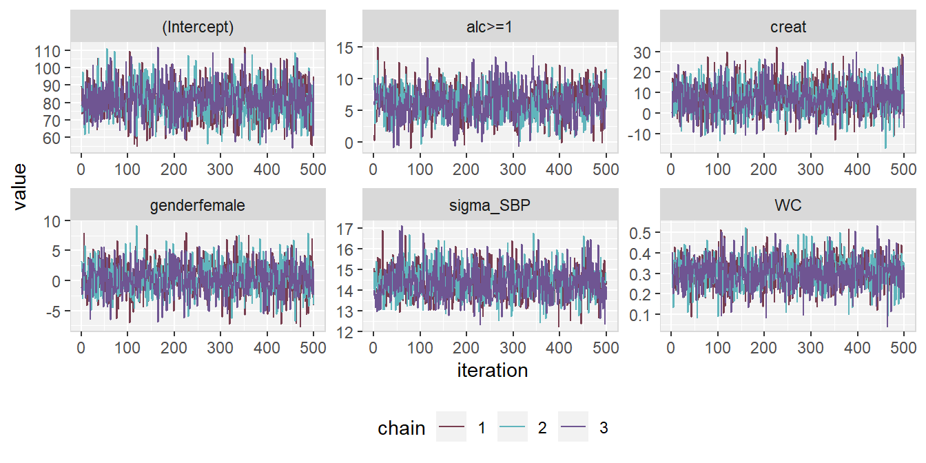
Figure 6.9: ggplot2 version of the traceplot of mod13a.
Densityplot
The posterior distributions can also be visualized using the function densplot(),
which plots the empirical density per node per chain, or combining chains
(when joined = TRUE).
The argument vlines takes a list of lists, containing specifications passed
to the function abline() (from package graphics which is available
with base R),
and allows the addition of (vertical) lines to the plot, e.g., marking zero,
or marking the posterior mean and 2.5% and 97.5% quantiles (Figure 6.10).
densplot(mod13a, ncol = 3,
         vlines = list(list(v = summary(mod13a)$stats[, "Mean"], lty = 1,
                            lwd = 2),
                       list(v = summary(mod13a)$stats[, "2.5%"], lty = 2),
                       list(v = summary(mod13a)$stats[, "97.5%"], lty = 2)
         )
)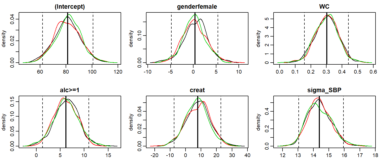
Figure 6.10: Densityplot of mod13a.
As with traceplot() it is possible to use the ggplot2 version of densplot()
when setting use_ggplot = TRUE. Here, vertical lines can be added as additional
layers.
Figure 6.11 shows, as an example, the posterior density
from mod13a to which vertical lines, representing the 95% credible interval
and a 95% confidence interval from a complete case analysis, are added.
The corresponding syntax is given in Appendix 6.B.
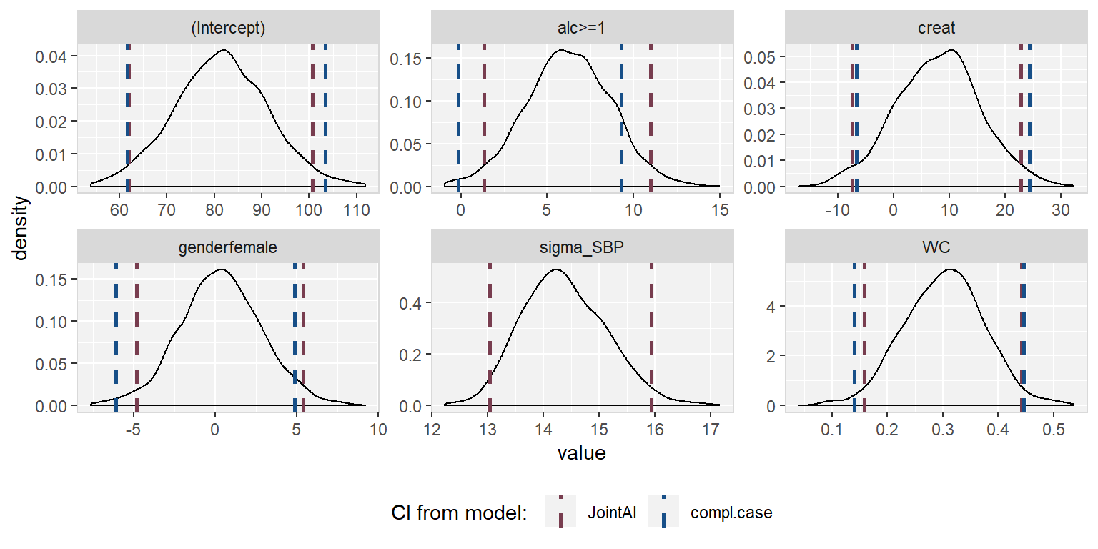
Figure 6.11: Densityplot of model mod13a.
6.7.2 Model Summary
A summary of the posterior distribution estimated in a JointAI model can be
obtained using the function summary().
The posterior summary consists of the mean, standard deviation and quantiles (by default the 2.5% and 97.5% quantiles) of the MCMC samples from all chains combined, as well as the tail probability (see below) and Gelman-Rubin criterion (see Section 6.7.3.1).
Additionally, some important characteristics of the MCMC samples on which the
summary is based, are given. This includes the range and number of iterations
(Sample size per chain), thinning interval and number of chains.
Furthermore, the number of observations (number of rows in the data) is printed.
##
##  Linear model fitted with JointAI
##
## Call:
## lm_imp(formula = SBP ~ gender + WC + alc + creat, data = NHANES,
##     n.iter = 500)
##
## Posterior summary:
##                Mean    SD   2.5%   97.5% tail-prob. GR-crit
## (Intercept)  81.368 9.844 61.972 100.732     0.0000    1.01
## genderfemale  0.353 2.541 -4.826   5.421     0.8907    1.01
## WC            0.302 0.073  0.159   0.441     0.0000    1.00
## alc>=1        6.219 2.456  1.321  10.984     0.0147    1.01
## creat         7.939 7.586 -7.465  22.848     0.2973    1.01
##
## Posterior summary of residual std. deviation:
##           Mean    SD 2.5% 97.5% GR-crit
## sigma_SBP 14.4 0.758   13  15.9       1
##
##
## MCMC settings:
## Iterations = 101:600
## Sample size per chain = 500
## Thinning interval = 1
## Number of chains = 3
##
## Number of observations: 186
For mixed models, summary() also returns the posterior summary of the
random effects covariance matrix D and the number of groups:
library(splines)
mod13b <- lme_imp(bmi ~ GESTBIR + ETHN + HEIGHT_M + ns(age, df = 3),
                  random = ~ ns(age, df = 3)|ID,
                  data = subset(simLong, !is.na(bmi)),
                  n.iter = 500, no_model = 'age')

summary(mod13b, start = 300)
## Linear mixed model fitted with JointAI
##
## Call:
## lme_imp(fixed = bmi ~ GESTBIR + ETHN + HEIGHT_M + ns(age, df = 3),
## data = subset(simLong, !is.na(bmi)), random = ~ns(age, df = 3) |
## ID, n.iter = 500, no_model = "age")
##
## Posterior summary:
## Mean SD 2.5% 97.5% tail-prob. GR-crit
## (Intercept) 16.31448 2.31751 11.9351 21.0625 0.000 1.06
## GESTBIR -0.03379 0.04371 -0.1258 0.0466 0.463 1.03
## ETHNother -0.00247 0.15991 -0.3029 0.3288 0.999 1.10
## HEIGHT_M 0.00545 0.00947 -0.0144 0.0247 0.560 1.04
## ns(age, df = 3)1 -0.30356 0.06287 -0.4186 -0.1834 0.000 3.12
## ns(age, df = 3)2 1.62073 0.19038 1.2633 1.9926 0.000 2.44
## ns(age, df = 3)3 -1.29077 0.06674 -1.4097 -1.1670 0.000 2.94
##
## Posterior summary of random effects covariance matrix:
## Mean SD 2.5% 97.5% tail-prob. GR-crit
## D[1,1] 1.439 0.1694 1.132 1.788 1.04
## D[1,2] -0.774 0.1126 -1.010 -0.573 0 1.18
## D[2,2] 0.735 0.0971 0.569 0.946 1.09
## D[1,3] -2.541 0.3590 -3.300 -1.873 0 1.07
## D[2,3] 2.424 0.2785 1.942 3.027 0 1.01
## D[3,3] 8.222 0.9635 6.549 10.314 1.08
## D[1,4] -0.741 0.1003 -0.957 -0.550 0 1.08
## D[2,4] 0.626 0.0743 0.492 0.783 0 1.04
## D[3,4] 2.096 0.2492 1.626 2.621 0 1.08
## D[4,4] 0.561 0.0767 0.422 0.717 1.22
##
## Posterior summary of residual std. deviation:
## Mean SD 2.5% 97.5% GR-crit
## sigma_bmi 0.457 0.00876 0.441 0.475 1
##
##
## MCMC settings:
## Iterations = 300:600
## Sample size per chain = 301
## Thinning interval = 1
## Number of chains = 3
##
## Number of observations: 1881
## Number of groups: 200The summary of parametric Weibull survival models also returns the summary of the posterior sample of the shape parameter of the Weibull distribution:
##
##  Weibull survival model fitted with JointAI
##
## Call:
## survreg_imp(formula = Surv(time, status) ~ age + sex + ph.karno +
##     meal.cal + wt.loss, data = lung, n.iter = 250)
##
## Posterior summary:
##                  Mean       SD      2.5%    97.5% tail-prob. GR-crit
## (Intercept)  5.58e+00 0.741546  4.19e+00 6.935742     0.0000    1.06
## age         -8.67e-03 0.007618 -2.38e-02 0.006025     0.2640    1.09
## sex2         4.22e-01 0.140230  1.39e-01 0.703982     0.0000    1.01
## ph.karno     9.28e-03 0.004567 -4.53e-05 0.018862     0.0533    1.05
## meal.cal     7.23e-05 0.000184 -2.59e-04 0.000426     0.7040    1.14
## wt.loss      1.69e-03 0.004738 -7.54e-03 0.011345     0.7413    1.00
##
## Posterior summary of the shape of the Weibull distribution:
##       Mean    SD 2.5% 97.5% GR-crit
## shape  1.3 0.081 1.13  1.45    1.05
##
##
## MCMC settings:
## Iterations = 101:350
## Sample size per chain = 250
## Thinning interval = 1
## Number of chains = 3
##
## Number of observations: 228
Tail Probability
The tail probability, calculated as \(2\times\min\left\{Pr(\theta > 0), Pr(\theta < 0)\right\},\) where \(\theta\) is the parameter of interest, is a measure of how likely the value 0 is under the estimated posterior distribution. Figure 6.12 visualizes three examples of posterior distributions and the corresponding minimum of \(Pr(\theta > 0)\) and \(Pr(\theta < 0)\) (shaded area).
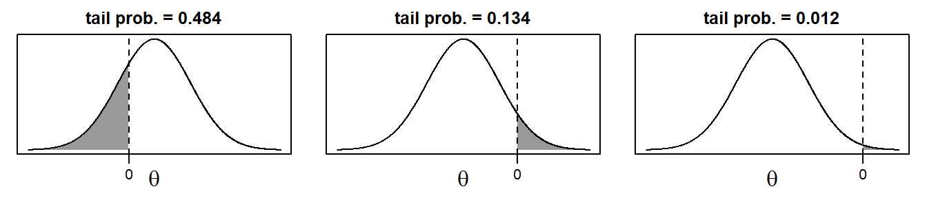
Figure 6.12: Visualization of the tail probability.
6.7.3 Evaluation Criteria
Convergence of the MCMC chains and precision of the posterior sample can also be evaluated in a more formal manner. Implemented in JointAI are the Gelman-Rubin criterion for convergence (Gelman and Rubin 1992; Brooks and Gelman 1998) and a comparison of the Monte Carlo Error with the posterior standard deviation.
6.7.3.1 Gelman-Rubin Criterion for Convergence
The Gelman-Rubin criterion (Gelman and Rubin 1992; Brooks and Gelman 1998),
also referred to as “potential scale reduction factor”,
evaluates convergence by comparing
within and between chain variability and, thus, requires at least two MCMC chains
to be calculated.
It is implemented for JointAI objects in the function GR_crit(), which
is based on the function gelman.diag() from the package coda (Plummer et al. 2006).
The upper limit of the confidence interval should not be much larger than 1.
## Potential scale reduction factors:
##
##              Point est. Upper C.I.
## (Intercept)        1.00       1.01
## genderfemale       1.00       1.01
## WC                 1.00       1.01
## alc>=1             1.01       1.03
## creat              1.00       1.00
## sigma_SBP          1.00       1.00
##
## Multivariate psrf
##
## 1.01
Besides the arguments start, end, thin, and subset, which are explained
in Section 6.7.4, GR_crit() also takes the arguments confidence,
transform and autoburnin of gelman.diag().
6.7.3.2 Monte Carlo Error
Precision of the MCMC sample can be checked with the function
MC_error().
It uses the function mcmcse.mat() from the package mcmcse (Flegal et al. 2017)
to calculate the Monte Carlo error (the error that is made since the sample
is finite) and compares is to the standard deviation of the posterior sample.
A rule of thumb is that the Monte Carlo error should not be more than 5% of the
standard deviation (Lesaffre and Lawson 2012).
Besides the arguments explained in Section 6.7.4, MC_error()
takes the arguments of mcmcse.mat().
##                est   MCSE    SD MCSE/SD
## (Intercept)  81.37 0.2896 9.844   0.029
## genderfemale  0.35 0.0750 2.541   0.029
## WC            0.30 0.0016 0.073   0.022
## alc>=1        6.22 0.0912 2.456   0.037
## creat         7.94 0.2387 7.586   0.031
## sigma_SBP    14.37 0.0222 0.758   0.029
MC_error() returns an object of class MCElist, which is a list containing
matrices with the posterior mean,
estimated Monte Carlo error, posterior standard deviation and the ratio of the
Monte Carlo error and posterior standard deviation, for the scaled
(if this MCMC sample was included in the JointAI object)
and unscaled (transformed back to the scale of the data) posterior samples.
The associated print method prints only the latter.
To facilitate quick evaluation of the Monte Carlo error to posterior standard
deviation ratio, plotting of an object of class MCElist using plot() shows
this ratio for each (selected) node and automatically adds a vertical line at
the desired cut-off (by default 5%; see Figure 6.13).
par(mar = c(3, 5, 0.5, 0.5), mgp = c(2, 0.6, 0), mfrow = c(1, 2))
plot(MC_error(mod13a))  # left panel
plot(MC_error(mod13a, end = 250))  # right panel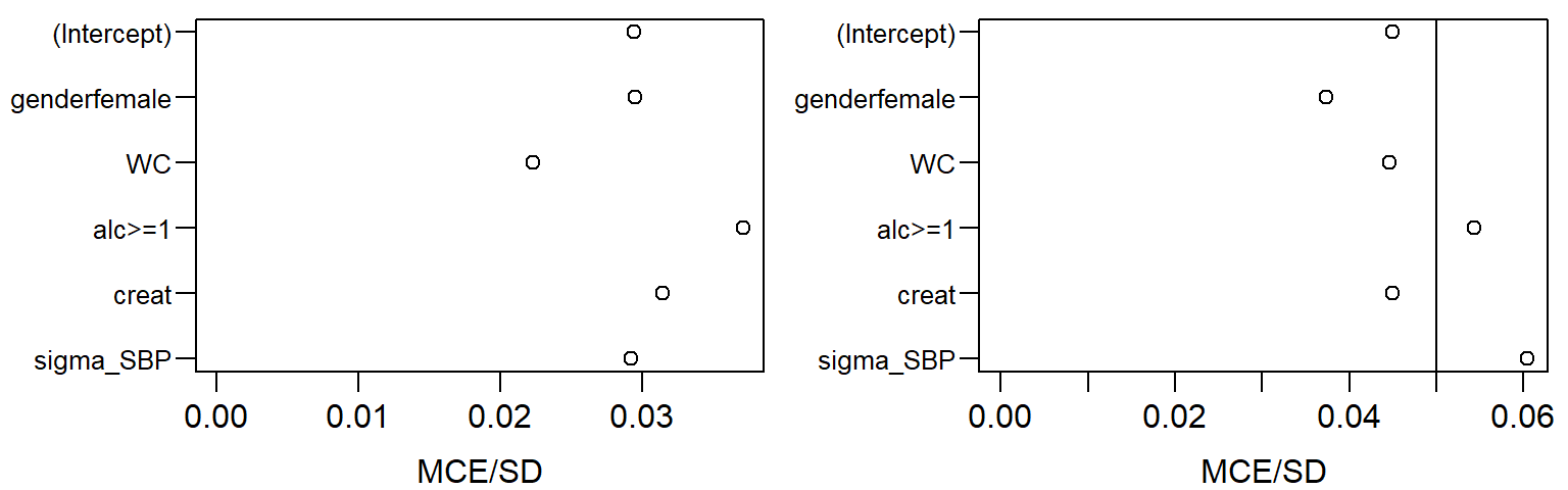
Figure 6.13: Plot of the MCElist object from mod13a. Left: including
all iterations, right: using only the first 250 iterations of the MCMC sample.
6.7.4 Subset of Output
By default, the functions traceplot(), densplot(), summary(), predict(),
GR_crit() and MC_Error() use all iterations of the MCMC sample and consider
only the parameters of the analysis model (if they were monitored).
In this section we describe how the
set of iterations and parameters/nodes to display can be changed using the
arguments subset, start, end and thin.
Subset of Parameters
When the main parameters of the analysis model have been monitored in a
JointAI object, i.e., when monitor_params was set to TRUE,
only these parameters are returned in the model summary, plots and criteria
shown above.
If the main parameters of the analysis model were not monitored and the
argument subset is not specified, all parameters that were monitored are
displayed.
To display output for nodes other than the main parameters of the analysis model
or for a subset of nodes, the argument subset needs to be specified.
6.7.4.0.1 Example:
To display only the parameters of the imputation models, we
set subset = c(analysis_main = FALSE, imp_pars = TRUE) (after re-estimating
the model with the monitoring for these parameters switched on):
mod13c <- update(mod13a, monitor_params = c(imp_pars = TRUE))
summary(mod13c, subset = c(analysis_main = FALSE, imp_pars = TRUE))
## Linear model fitted with JointAI
##
## Call:
## lm_imp(formula = SBP ~ gender + WC + alc + creat, data = NHANES,
## n.iter = 500, monitor_params = c(imp_pars = TRUE))
##
## Posterior summary:
## Mean SD 2.5% 97.5% tail-prob. GR-crit
## alpha[1] 0.1624 0.0990 -0.0327 0.3598 0.1000 1.00
## alpha[2] -0.3506 0.1484 -0.6414 -0.0557 0.0173 1.00
## alpha[3] 0.4901 0.0902 0.3078 0.6633 0.0000 1.01
## alpha[4] -1.0338 0.1331 -1.2930 -0.7647 0.0000 1.01
## alpha[5] 0.0775 0.0666 -0.0522 0.2084 0.2587 1.00
## alpha[6] -0.1277 0.2449 -0.6010 0.3807 0.5880 1.01
## alpha[7] -0.8928 0.4133 -1.6684 -0.0750 0.0320 1.01
## alpha[8] 0.0887 0.1769 -0.2568 0.4329 0.6373 1.01
## alpha[9] -0.2627 0.2086 -0.6772 0.1529 0.2080 1.00
## tau_WC 1.0280 0.1083 0.8277 1.2551 0.0000 1.01
## tau_creat 1.3997 0.1525 1.1064 1.7261 0.0000 1.01
##
##
## MCMC settings:
## Iterations = 101:600
## Sample size per chain = 500
## Thinning interval = 1
## Number of chains = 3
##
## Number of observations: 186Example:
To select only some of the parameters, they can be specified directly by
name via the other element of subset.
Example:
This also works when a subset of the imputed values should be displayed:
# re-fit the model and monitor the imputed values
mod13d <- lm_imp(SBP ~ gender + age + albu + occup + alc, n.iter = 200,
                 data = NHANES, monitor_params = c(imps = TRUE))

# select all imputed values for 'albu' (4th column of Xc)
sub3 <- grep('Xc\\[[[:digit:]]+,4\\]', parameters(mod13d), value = TRUE)
sub3
## [1] "Xc[10,4]" "Xc[14,4]" "Xc[18,4]" "Xc[25,4]" "Xc[80,4]" "Xc[118,4]"
## [7] "Xc[172,4]" "Xc[180,4]"Example:
When the number of imputed values is large or in order to check convergence of random effects, it may not be feasible to plot and inspect all traceplots. In that case, a random subset of, for instance, the random effects, can be selected (output not shown):
# re-fit the model monitoring the random effects
mod13e <- update(mod13a, monitor_params = c(ranef = TRUE))

# extract random intercepts and random slopes
ri <- grep('^b\\[[[:digit:]]+,1\\]$', colnames(mod13e$MCMC[[1]]),
           value = TRUE)
rs <- grep('^b\\[[[:digit:]]+,2\\]$', colnames(mod13e$MCMC[[1]]),
           value = TRUE)

# to plot the chains of 12 randomly selected random intercepts & slopes:
traceplot(mod13e, subset = list(other = sample(ri, size = 12)), ncol = 4)
traceplot(mod13e, subset = list(other = sample(rs, size = 12)), ncol = 4)
6.7.4.1 Subset of MCMC Samples
With the arguments start, end and thin it is possible to
select which iterations from the MCMC sample are included in the summary.
start and end specify the first and last iterations to be used,
thin the thinning interval. Specification of start thus allows the user to discard
a “burn-in”, i.e., the iterations before the MCMC chain had converged.
6.7.5 Predicted Values
Often, the aim of an analysis is not only to estimate the association between outcome and covariates but to predict future outcomes or outcomes for new subjects.
The function predict() allows us to obtain predicted values and corresponding
credible intervals from JointAI objects. Note that for mixed
models, currently only marginal prediction is implemented, not prediction conditional on
the random effects.
A dataset containing data for which the prediction should be performed for is specified
via the argument newdata. The argument quantiles allows specification of the
quantiles of the posterior sample that are used to obtain the prediction interval
(by default the 2.5% and 97.5% quantile).
Arguments start, end and thin control the subset of MCMC samples used.
## $dat
##          SBP gender age             race   WC alc educ creat albu uricacid
## 392 126.6667   male  32 Mexican American 94.1  <1  low  0.83  4.2      8.7
##     bili occup  smoke      fit     2.5%    97.5%
## 392    1  <NA> former 116.3997 112.5729 120.2564
##
## $fit
## [1] 116.3997
##
## $quantiles
##           [,1]
## 2.5%  112.5729
## 97.5% 120.2564
predict() returns a list with elements dat (a dataset consisting of
newdata with the predicted values and quantiles appended),
fit (the predicted values) and quantiles (the quantiles that form the
prediction interval).
Prediction to Visualize Non-linear Effects
Another reason to obtain predicted values is the visualization of non-linear
effects (see Figure 6.14).
To facilitate the generation of a dataset for such a prediction,
the function predDF() can be used. It generates a data.frame
that contains a sequence of values through the range of observed values for a
covariate specified by the argument var, and the median or reference value for
all other continuous and categorical variables.
# create dataset for prediction
newDF <- predDF(mod13b, var = "age")

# obtain predicted values
pred <- predict(mod13b, newdata = newDF, start = 300)

# plot predicted values and prediction interval
matplot(pred$dat$age, pred$dat[, c('fit', '2.5%', '97.5%')],
        lty = c(1,2,2), type = 'l', col = 1,
        xlab = 'age in months', ylab = 'predicted value')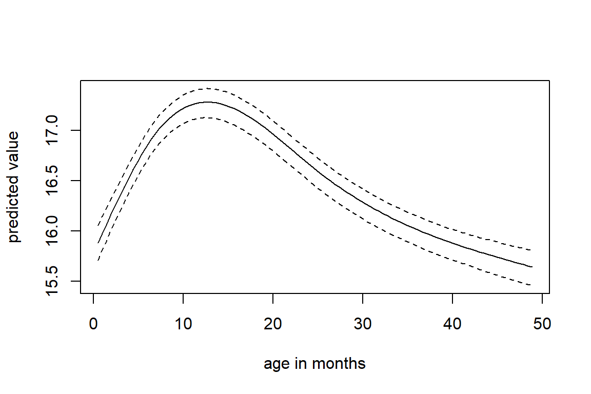
Figure 6.14: Predicted values of BMI and corresponding 95% credible intervals from mod13b.
6.7.6 Export of Imputed Values
Imputed datasets can be extracted from a JointAI object (in which a monitor for
the imputed values has been set, i.e., monitor_params = c(imps = TRUE))
with the function get_MIdat().
A completed dataset is created by taking the imputed values from a randomly chosen iteration of the MCMC sample, transforming them back to the original scale (if scaling was performed before the MCMC sampling) and filling them into the original incomplete data.
The argument m specifies the number of imputed datasets to be created,
include controls whether the original data are included in the long format
data.frame (default is include = TRUE),
start specifies the first iteration that may be used,
and minspace is the minimum number of iterations between
iterations eligible for selection.
To make the selection of iterations reproducible, a
seed value can be specified via the argument seed.
When export_to_SPSS = TRUE the imputed data is exported to SPSS
(IBM SPSS Statistics, IBM Corp.), i.e.,
a .txt file containing the data and a .sps file containing SPSS syntax to
convert the data into an SPSS data file (with ending .sav) are written.
Arguments filename and resdir allow specification of the name of the .txt and
.sps file and the directory they are written to.
get_MIdat() returns a long-format data.frame containing the imputed datasets
(and by default the original data) stacked on top of each other. The imputation number
is given in the variable Imputation_, column .id contains a newly created
id variable for each observation in cross-sectional data (multi-level data should
already contain an id variable) and the column .rownr identifies rows of the
original data (which is relevant in multi-level data).
The function plot_imp_distr() allows visual comparison of the
distributions of the observed and imputed values (Figure 6.15).
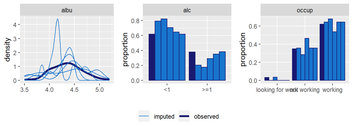
Figure 6.15: Distribution of observed and imputed values from mod13d.
6.8 Assumptions and Extensions
Like any statistical model, the approach to imputation followed in JointAI relies on assumptions that need to be satisfied in order to obtain valid results.
A commonly made assumption that is also required for JointAI is that the missing data mechanism is ignorable, i.e., that data is Missing At Random (MAR) or Missing Completely At Random (MCAR) (Rubin 1976,) and that parameters in the model of the missingness mechanism are independent of the parameters in the data model (Schafer 1997). It is the task of the researcher to critically evaluate whether this assumption is satisfied for a given dataset and model.
Furthermore, all models involved in the imputation and analysis need to be
correctly specified. In current implementations of imputation procedures in
software, imputation models are typically automatically specified, using
standard assumptions like linear associations and default model types.
In JointAI, the arguments models and auxvar permit tailoring of the
automatically chosen models to some extent, by allowing the user to chose non-normal
imputation models for continuous variables and to include variables or functional
forms of variables in the linear predictor of the imputation models that are
not used in the analysis model.
When using auxiliary variables in JointAI, it should be noted that due to the ordering of the conditional distributions in the sequence of models it is implied that the auxiliary variable is independent of the outcome, since neither the model for the auxiliary variable (if the auxiliary variable has missing values) has the outcome in its linear predictor nor vice versa.
Moreover, in order to make software usable, default values have to be chosen for various parameters. These default values are chosen to work well in certain settings, but can not be guaranteed to be appropriate in general and it is the task of the user to make the appropriate changes. In JointAI this concerns, for example, the choice of hyperparameters and automatically chosen types of imputation models.
To expand the range of settings in which JointAI provides a valid and user-friendly way to simultaneously analyse and impute data, several extensions are planned, for example:
Implement the use of (penalized) splines for incompletely observed covariates, thereby improving model fit.
Increase the flexibility of imputation models by optional inclusion of interaction terms and non-parametric Bayesian models that allow imputation under non-standard distributions.
Evaluation of model fit of the analysis and imputation models to help the user prevent bias due to misspecification.
Implementation of subject-specific prediction from mixed models.
Extend the analysis models to handle endogenous covariates by modelling random effects (and error terms) jointly.
Appendix
6.A Default Hyperparameters
## $norm
##    mu_reg_norm   tau_reg_norm shape_tau_norm  rate_tau_norm
##          0e+00          1e-04          1e-02          1e-02
##
## $gamma
##    mu_reg_gamma   tau_reg_gamma shape_tau_gamma  rate_tau_gamma
##           0e+00           1e-04           1e-02           1e-02
##
## $beta
##    mu_reg_beta   tau_reg_beta shape_tau_beta  rate_tau_beta
##          0e+00          1e-04          1e-02          1e-02
##
## $logit
##  mu_reg_logit tau_reg_logit
##         0e+00         1e-04
##
## $poisson
##  mu_reg_poisson tau_reg_poisson
##           0e+00           1e-04
##
## $probit
##  mu_reg_probit tau_reg_probit
##          0e+00          1e-04
##
## $multinomial
##  mu_reg_multinomial tau_reg_multinomial
##               0e+00               1e-04
##
## $ordinal
##    mu_reg_ordinal   tau_reg_ordinal  mu_delta_ordinal tau_delta_ordinal
##             0e+00             1e-04             0e+00             1e-04
##
## $Z
## function (nranef)
## {
##     if (nranef > 1) {
##         RinvD <- diag(as.numeric(rep(NA, nranef)))
##         KinvD <- nranef
##     }
##     else {
##         RinvD <- KinvD <- NULL
##     }
##     list(RinvD = RinvD, KinvD = KinvD, shape_diag_RinvD = 0.1,
##         rate_diag_RinvD = 0.01)
## }
## <bytecode: 0x000000001d177070>
## <environment: 0x000000001d173e10>
##
## $surv
##  mu_reg_surv tau_reg_surv
##        0.000        0.001
##
## $coxph
##     c     r   eps
## 1e-03 1e-01 1e-10
6.B Density Plot using ggplot2
# fit the complete-case version of the model
mod13a_cc <- lm(formula(mod13a), data = NHANES)


# make a dataset containing the quantiles of the posterior sample and
# confidence intervals from the complete case analysis:
quantDF <- rbind(data.frame(variable = rownames(summary(mod13a)$stat),
                            type = '2.5%',
                            model = 'JointAI',
                            value = summary(mod13a)$stat[, c('2.5%')]
                            ),
                 data.frame(variable = rownames(summary(mod13a)$stat),
                            type = '97.5%',
                            model = 'JointAI',
                            value = summary(mod13a)$stat[, c('97.5%')]
                 ),
                 data.frame(variable = names(coef(mod13a_cc)),
                            type = '2.5%',
                            model = 'cc',
                            value = confint(mod13a_cc)[, '2.5 %']
                 ),
                 data.frame(variable = names(coef(mod13a_cc)),
                            type = '97.5%',
                            model = 'cc',
                            value = confint(mod13a_cc)[, '97.5 %']
                 )
)


# ggplot version:
p13a <- densplot(mod13a, ncol = 3, use_ggplot = TRUE, joined = TRUE) +
  theme(legend.position = 'bottom',
        panel.background = element_rect(fill = grey(0.95)),
        panel.border = element_rect(fill = NA, color = grey(0.85)),
        strip.background = element_rect(color = grey(0.85)))


# add vertical lines for the:
# - confidence intervals from the complete case analysis
# - quantiles of the posterior distribution
p13a +
  geom_vline(data = quantDF, aes(xintercept = value, color = model),
             lty = 2, lwd = 1) +
  scale_color_manual(name = 'CI from model: ',
                     limits = c('JointAI', 'cc'),
                     values = c("#783D4F", "#174F88"),
                     labels = c('JointAI', 'compl.case'))
red <- function(x) {
x <- rlang::enexpr(x)
if (knitr:::is_latex_output()) {
paste0("\\textcolor{red}{", x, "}")
} else {
paste0("<span style='color:red'>", x, "</span>")
}
}
R <- function() {
if (knitr:::is_latex_output()) {
'\\textsf{R}'
} else {
'R'
}
}
JAGS <- function() {
if (knitr:::is_latex_output()) {
'\\textsf{JAGS}'
} else {
'JAGS'
}
}
WinBUGS <- function() {
if (knitr:::is_latex_output()) {
'\\textsf{WinBUGS}'
} else {
'WinBUGS'
}
}References
Bartlett, Jonathan W., Shaun R. Seaman, Ian R. White, and James R. Carpenter. 2015. “Multiple Imputation of Covariates by Fully Conditional Specification: Accommodating the Substantive Model.” Statistical Methods in Medical Research 24 (4): 462–87. https://doi.org/10.1177/0962280214521348.
Brooks, Stephen P., and Andrew Gelman. 1998. “General Methods for Monitoring Convergence of Iterative Simulations.” Journal of Computational and Graphical Statistics 7 (4): 434–55. https://doi.org/10.1080/10618600.1998.10474787.
Corporation, Microsoft, and Steve Weston. 2018. DoParallel: Foreach Parallel Adaptor for the ’Parallel’ Package. https://CRAN.R-project.org/package=doParallel.
Erler, Nicole S. 2019. JointAI: Joint Analysis and Imputation of Incomplete Data. https://github.com/nerler/JointAI.
Erler, Nicole S., Dimitris Rizopoulos, Vincent W. V. Jaddoe, Oscar H. Franco, and Emmanuel M. E. H. Lesaffre. 2019. “Bayesian Imputation of Time-Varying Covariates in Linear Mixed Models.” Statistical Methods in Medical Research 28 (2): 555–88. https://doi.org/10.1177/0962280217730851.
Erler, Nicole S., Dimitris Rizopoulos, Joost van Rosmalen, Vincent W. V. Jaddoe, Oscar H. Franco, and Emmanuel M. E. H. Lesaffre. 2016. “Dealing with Missing Covariates in Epidemiologic Studies: A Comparison Between Multiple Imputation and a Full Bayesian Approach.” Statistics in Medicine 35 (17): 2955–74. https://doi.org/10.1002/sim.6944.
Flegal, James M., John Hughes, Dootika Vats, and Ning Dai. 2017. Mcmcse: Monte Carlo Standard Errors for Mcmc. Riverside, CA, Denver, CO, Coventry, UK,; Minneapolis, MN.
Gelman, Andrew, and Donald B. Rubin. 1992. “Inference from Iterative Simulation Using Multiple Sequences.” Statistical Science 7 (4): 457–72. https://doi.org/10.1214/ss/1177011136.
Ibrahim, Joseph G., Ming-Hui Chen, and Stuart R. Lipsitz. 2002. “Bayesian Methods for Generalized Linear Models with Covariates Missing at Random.” Canadian Journal of Statistics 30 (1): 55–78. https://doi.org/10.2307/3315865.
Lesaffre, Emmanuel M. E. H., and Andrew B. Lawson. 2012. Bayesian Biostatistics. John Wiley & Sons. https://doi.org/10.1002/9781119942412.
Lunn, David, Chris Jackson, Nicky Best, David Spiegelhalter, and Andrew Thomas. 2012. The BUGS book: A practical introduction to Bayesian analysis. Chapman; Hall/CRC.
Microsoft, and Steve Weston. 2017. Foreach: Provides Foreach Looping Construct for R. https://CRAN.R-project.org/package=foreach.
National Center for Health Statistics (NCHS). 2011. “National Health and Nutrition Examination Survey Data.” U.S. Department of Health and Human Services, Centers for Disease Control and Prevention. https://www.cdc.gov/nchs/nhanes/.
Novo, Alvaro A., and Joseph L. Schafer. 2010. Norm: Analysis of Multivariate Normal Datasets with Missing Values. (version R package version 1.0-9.5.). http://CRAN.R-project.org/package=norm.
Pinheiro, Jose, Douglas Bates, Saikat DebRoy, Deepayan Sarkar, and R Core Team. 2018. nlme: Linear and Nonlinear Mixed Effects Models. https://CRAN.R-project.org/package=nlme.
Plummer, M. 2003. “JAGS: A Program for Analysis of Bayesian Graphical Models Using Gibbs Sampling.” Edited by Kurt Hornik, Friedrich Leisch, and Achim Zeileis.
Plummer, Martyn. 2018. Rjags: Bayesian Graphical Models Using Mcmc. https://CRAN.R-project.org/package=rjags.
Plummer, Martyn, Nicky Best, Kate Cowles, and Karen Vines. 2006. “CODA: Convergence Diagnosis and Output Analysis for Mcmc.” R News 6 (1): 7–11. https://journal.r-project.org/archive/.
R Core Team. 2018. R: A Language and Environment for Statistical Computing. Vienna, Austria: R Foundation for Statistical Computing. https://www.R-project.org/.
Rubin, Donald B. 1976. “Inference and Missing Data.” Biometrika 63 (3): 581–92. https://doi.org/10.2307/2335739.
Rubin, Donald B. 1987. Multiple Imputation for Nonresponse in Surveys. Wiley Series in Probability and Statistics. Wiley. https://doi.org/10.1002/9780470316696.
Rubin, Donald B. 2004. “The Design of a General and Flexible System for Handling Nonresponse in Sample Surveys.” The American Statistician 58 (4): 298–302. https://doi.org/10.1198/000313004X6355.
Schafer, Joseph L. 1997. Analysis of Incomplete Multivariate Data. Chapman & Hall/Crc Monographs on Statistics & Applied Probability. Taylor & Francis.
Terry M. Therneau, and Patricia M. Grambsch. 2000. Modeling Survival Data: Extending the Cox Model. New York: Springer.
Therneau, Terry M. 2015. A Package for Survival Analysis in S. https://CRAN.R-project.org/package=survival.
Van Buuren, Stef. 2012. Flexible Imputation of Missing Data. Chapman & Hall/CRC Interdisciplinary Statistics. Taylor & Francis.
Van Buuren, Stef, and Karin Groothuis-Oudshoorn. 2011. “mice: Multivariate Imputation by Chained Equations in R.” Journal of Statistical Software 45 (3): 1–67. https://doi.org/10.18637/jss.v045.i03.
White, Ian R., Patrick Royston, and Angela M. Wood. 2011. “Multiple imputation using chained equations: Issues and guidance for practice.” Statistics in Medicine 30 (4): 377–99. https://doi.org/10.1002/sim.4067.
Wickham, Hadley. 2016. Ggplot2: Elegant Graphics for Data Analysis. Springer-Verlag New York. http://ggplot2.org.