Chapter 2 Dealing with Missing Covariates in Epidemiologic Studies

---

This chapter is based on

Nicole S. Erler, Dimitris Rizopoulos, Joost van Rosmalen, Vincent W. V. Jaddoe, Oscar H. Franco and Emmanuel M. E. H. Lesaffre. Dealing with missing covariates in epidemiologic studies: a comparison between multiple imputation and a full Bayesian approach. Statistics in Medicine, 2016; 35(17), 2955 – 2974. doi:10.1002/sim.6944

Abstract

Incomplete data are generally a challenge to the analysis of most large studies. The current gold standard to account for missing data is multiple imputation (MI), and more specifically multiple imputation with chained equations (MICE). Numerous studies have been conducted to illustrate the performance of MICE for missing covariate data. The results show that the method works well in various situations. However, less is known about its performance in more complex models, specifically when the outcome is multivariate as in longitudinal studies. In current practice, the multivariate nature of the longitudinal outcome is often neglected in the imputation procedure or only the baseline outcome is used to impute missing covariates. In this chapter, we evaluate the performance of MICE using different strategies to include a longitudinal outcome into the imputation models and compare it with a fully Bayesian approach that jointly imputes missing values and estimates the parameters of the longitudinal model. Results from simulation and a real data example show that MICE requires the analyst to correctly specify which components of the longitudinal process need to be included in the imputation models in order to obtain unbiased results. The fully Bayesian approach, on the other hand, does not require the analyst to explicitly specify how the longitudinal outcome enters the imputation models. It performed well under different scenarios.

2.1 Introduction

Missing values are a common complication in the analysis of cohort studies. Since epidemiologic studies are often adjusted for a large number of possible confounders, the treatment of missing covariate values is of special interest and our focus in this chapter. There have been numerous publications that show that naive ways to handle missing data, like complete case analysis, often lead to biased estimates and considerable loss of power (Molenberghs and Kenward 2007; Donders et al. 2006; Janssen et al. 2010; Knol et al. 2010; Sterne et al. 2009; Van Buuren 2012).

One standard approach to tackle this problem is to perform multiple imputation (MI) (Rubin 1987). Among the different flavours of MI, the Multiple Imputation with Chained Equations (MICE) (Van Buuren 2012) approach has gained the widest acceptance due to its good performance and ease of use. MI, and hence also MICE, works in three steps: First, a small number (often 5 or 10) of datasets are created by imputing each missing value multiple times. Each of the completed datasets can then be analysed using standard complete data methods. To obtain the overall result and to take additional uncertainty created by the missing values into account, the derived estimates are being pooled in the last step.

As a consequence of the separation of imputation and analysis steps, the relations between the outcome and the covariates, which are modelled in the analysis step, must be included explicitly in these imputation models. This means that the imputation models should not only contain other covariates in the predictor but also the outcome (Moons et al. 2006). When the outcome is univariate (and the model does not contain non-linear effects or interactions that involve incomplete covariates) this can be easily done because the outcome is just one of the variables in the dataset. However, when the outcome has a multivariate nature, such as the longitudinal outcome in our motivating study, it is not directly evident how this can be achieved, since longitudinal outcomes are often unbalanced with different subjects providing a different number of measurements at different time points. To overcome this problem one could consider simple or complex summaries of the long trajectories, such as including only a single value (e.g., baseline or the last available one) or the area under the trajectory. However, it is not clear which of these representations is the most adequate one for a specific analysis model and moreover, except in very simple situations, these summaries discard relevant information. As will be shown later, inclusion of inadequate summary measures of the subjects’ trajectories can lead to bias.

To prevent the problem of having to specify the appropriate summary measure in the MICE approach we propose here a fully Bayesian approach which combines the analysis model with the imputation models. The essential difference to MICE is that by combining the imputation and analysis in one estimation procedure, the Bayesian approach obtains inferences on the posterior distribution of the parameters and missing covariates directly and jointly. Thereby, the whole trajectory of the longitudinal outcome is implicitly taken into account in the imputation of missing covariate values and no summary representation is necessary. A common approach to specify the joint distribution is to assume (latent) normal distributions for all variables and model it as multivariate normal (Carpenter and Kenward 2013; Goldstein et al. 2009). In the present work, we chose a different approach and follow Ibrahim, Chen, and Lipsitz (2002), who propose a decomposition of the likelihood into a series of univariate conditional distributions. This produces the sequential fully Bayesian (SFB) approach which is a flexible and easy to implement alternative to MICE. Furthermore, since missing values are continuously imputed in each iteration of the estimation procedure, the uncertainty about the missing values is automatically taken into account and no pooling is necessary.

Besides approaches using multiple imputation or the fully Bayesian framework, other methods that can handle missing covariates in longitudinal settings have been investigated in the literature. Stubbendick and Ibrahim (2003), for instance, approach the missing data problem using a likelihood-based approach that factorized the joint likelihood into a sequence of conditional distributions, analogue the SFB approach. Other authors (Chen, Grace, and Cook 2010; Chen and Zhou 2011) have shown how to apply weighted estimating equations for inference in settings with incomplete data.

In the present study, we describe different strategies to include a longitudinal outcome in MICE and compare them with the SFB approach. Both methods were evaluated using simulation and a motivating real data example that required the analysis of a large dataset with missing values in several variables of different types. The rest of this chapter is organized as follows: Section 2.2 briefly describes the data motivating this study. In Section 2.3 we introduce the problem of missing data, and describe and compare the two methods of interest, MICE and the SFB approach. Both methods are applied to a real data example in Section 2.4 and evaluated in a simulation study, which is described in Section 2.5. Section 2.6 concludes the chapter with a discussion.

2.2 Generation R Data

We have taken a subset of variables measured within the Generation R Study, a population-based prospective cohort study from early fetal life onwards in Rotterdam, the Netherlands (Jaddoe et al. 2012), to illustrate both approaches. It was extracted with the aim to analyse the effect of diet, represented by three principal components, on gestational weight gain and contains a number of incomplete covariates of mixed type. The relationship between diet and weight gain during pregnancy is of special interest to epidemiologists because diet may influence the amount of weight gained during pregnancy and subsequently affect the risk of adverse pregnancy outcomes. Furthermore, the Body Mass Index (BMI) before pregnancy is an important related factor on which general guidelines and recommendations for gestational weight gain are based.

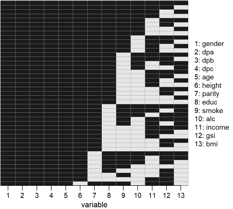
Figure 2.1: Missing data pattern of the Generation R data.

In the present study, data of 3374 pregnant women for whom dietary information was available, were analysed. Each woman was asked for her pre-pregnancy weight (baseline) and had up to three weight measurements during pregnancy, one in each trimester. There were 2297 women for whom all four weight measurements were recorded, 917 for whom three weight measurements were observed, 146 women had two measurements, and 14 women had only one measurement of weight. The gestational age at each measurement was recorded and the time point of the baseline measurement was set to be zero for all women. Table 2.1 in Appendix 2.A gives an overview of the available data. All covariates are cross-sectional. The variable bmi was calculated from baseline weight (weight0) and height. Except for gender, age and the dietary pattern variables, all variables had missing values, in proportions ranging between 0.03% and 14.17%. Reasons for missing covariate values in this study are usually (item) non-response in the questionnaires used. Missing baseline weight or weight measurement in the first trimester occurs when women are included in the study at a later gestational age. The missing pattern of the covariates is visualized in Figure 2.1. Variables 2 – 6, 12 and 13 are continuous, variables 1, 7 and 11 are binary and variables 8 – 10 are categorical with three categories each. 2236 individuals had complete covariate data.

2.3 Dealing with Missing Data

A standard modelling framework for studying the relationship between a longitudinal outcome \(\mathbf y\) and predictor variables \(\mathbf X\) is a linear mixed model: \[ y_{ij} = \mathbf x_{ij}^\top\boldsymbol\beta + \mathbf z_{ij}^\top\mathbf b_i + \varepsilon_{ij}, \] where \(y_{ij}\) is the \(j\)-th observation of individual \(i\), measured at time \(t_{ij}\), \(\boldsymbol\beta\) denotes the vector of regression coefficients of the design matrix of the fixed effects \(\mathbf X_i\), where \(\mathbf x_{ij}\) is a column vector that contains the \(j\)-th row of that matrix, and, analogously, \(z_{ij}\) denotes a row of the design matrix \(\mathbf Z_i\) of the random effects \(\mathbf b_i\) and contains a subset of the variables in \(x_{ij}\). Furthermore, the vector \(\mathbf b_i\) follows a multivariate normal distribution with mean zero and covariance matrix \(\mathbf D\), and \(\varepsilon_{ij}\) is an error term that is normally distributed with mean zero and variance \(\sigma_y^2\).

In a complete data setting, the probability density function of interest is \(p(y_{ij} \mid \mathbf x_{ij}, \mathbf z_{ij}, \boldsymbol\theta_{Y\mid X})\), where \(\boldsymbol\theta_{Y\mid X}\) denotes the vector of parameters of the model. When some of the covariates are incomplete, \(\mathbf X\) consists of two parts, the completely observed variables \(\mathbf X_{obs}\) and those variables that containing missing values, \(\mathbf X_{mis}\). The measurement model \(p(y_{ij} \mid \mathbf x_{ij,obs}, \mathbf x_{ij, mis}, \mathbf z_{ij}, \boldsymbol\theta_{Y\mid X})\) then depends on unobserved data and standard complete data methods cannot be used any more.

In this chapter, we restrict our attention to the imputation of cross-sectional covariates. The missing data mechanism of the outcome is assumed to be ignorable, i.e., Missing At Random (MAR) or Missing Completely at Random (MCAR) (Little and Rubin 2002; Seaman et al. 2013), and hence the missing outcome values do not require special treatment when using mixed effects models.

2.3.1 Multiple Imputation using Chained Equations

The underlying principle of MI is to divide the analysis of incomplete data into three steps: imputation, analysis and pooling. MICE is a popular implementation of the imputation step since it allows for multivariate missing data and does not require a specific missingness pattern. The idea behind MICE is that, under certain regularity conditions, the multivariate distribution \[\begin{equation} p(\mathbf x_{i,mis} \mid \mathbf y_i, \mathbf x_{i,obs}, \boldsymbol\theta_{X}), \tag{2.1} \end{equation}\] with \(\mathbf x_{i,mis} = (x_{i,mis_1}, \ldots, x_{i,mis_p})^\top\) and \(\mathbf x_{i,obs} = (x_{i,obs_1}, \ldots, x_{i,obs_q})^\top\), can be uniquely determined by its full conditional distributions and hence Gibbs sampling of the conditional distributions can be used to produce a sample from (2.1) (Van Buuren 2012). However, the MICE procedure does not actually start from a specification of (2.1), but it directly defines a series of conditional, predictive models of the form \[\begin{equation} p(x_{i, mis_\ell} \mid \mathbf x_{i,mis_{-\ell}}, \mathbf x_{i,obs}, \mathbf y_i, \boldsymbol\theta_{X_\ell}),\tag{2.2} \end{equation}\] that link each incomplete predictor variable \(x_{i, mis_\ell}, \; \ell=1,\ldots,p\), with other incomplete and complete predictors, \(\mathbf x_{i,mis_{-\ell}}\) and \(\mathbf x_{i,obs}\), respectively, and importantly with the outcome. These predictive distributions are typically members of the extended exponential family (extended with models for ordinal data) with linear predictor \[ g_{\ell}\left\{E\left(x_{i,mis_{\ell}}\mid x_{i,obs}, x_{i,mis_{-\ell}}, \mathbf y_i, \boldsymbol\gamma_\ell, \boldsymbol\xi_\ell, \boldsymbol\alpha_\ell\right)\right\} = \boldsymbol \gamma^\top_{\ell}\mathbf x_{i,obs} + \boldsymbol\xi_{\ell}^\top \mathbf x_{i, mis_{-\ell}} + \boldsymbol \alpha_{\ell}^\top f(\mathbf y_i), \] where \(g_\ell(\cdot)\) is the one-to-one monotonic link function for the \(\ell\)-th covariate and \(\boldsymbol \gamma_\ell\), \(\boldsymbol \xi_\ell\) and \(\boldsymbol \alpha_\ell\) are vectors of parameters relating the complete and missing covariates and the outcome to \(x_{i, mis_\ell}\).

The function \(f(\cdot)\) specifies how the outcome enters the linear predictor. In the univariate case, the default choice for \(f(y_i)\) is simply the identity function. However, when we have a multivariate \(\mathbf y_i\), such as a longitudinal outcome, we cannot always simply specify \(\boldsymbol\alpha_\ell^\top \mathbf y_i\) because \(\mathbf y_i\) may have different length than \(\mathbf y_k\) for \(i\neq k\), and the time points \(t_{ij}\) and \(t_{kj}\) of the observations \(y_{ij}\) and \(y_{kj}\) may be very different. Hence, it is not meaningful to use the same regression coefficient \(\alpha_{\ell j}\) to connect outcomes of different individuals with \(x_{i, mis_{\ell}}\) and a representation needs to be found that summarizes \(\mathbf y_i\) and that has the same number of elements which also have the same interpretation for all individuals.

Some examples for \(f(\mathbf y_i)\) could be \[\begin{eqnarray} f(\mathbf y_i) &=& 0, \tag{2.3}\\ f(\mathbf y_i) &=& y_{ij}, \tag{2.4}\\ f(\mathbf y_i) &=& \frac{1}{n_i}\sum_{j=1}^{n_i} y_{ij}, \tag{2.5}\\ f(\mathbf y_i) &=& \sum_{j=1}^{n_i-1} (t_{ij+1}-t_{ij}) \frac{y_{ij} + y_{ij+1}}{2}, \tag{2.6}\\ f(\mathbf y_i) &=& \mathbf{\hat b}_{i} = \mathbf{\widehat D}\mathbf{\widetilde Z}_i^\top \left(\mathbf{\widetilde Z}_i \mathbf{\widehat D} \mathbf{\widetilde Z}_i^\top + \boldsymbol{\widehat\Sigma}_i \right)^{-1} \left(\mathbf y_i - \mathbf{\widetilde X}_i\boldsymbol{\hat\beta}\right), \tag{2.7}\\ f(\mathbf y_i) &=& \int \mathbf{\widetilde X}_i(t) \boldsymbol{ \hat \beta} + \mathbf{\widetilde Z}_i(t) \mathbf{\hat b}_i \;dt. \tag{2.8} \end{eqnarray}\]

Here, \(f(\mathbf y_i)\) from (2.3) results in omitting the outcome completely from the imputation procedure. Equations (2.4) – (2.6) are examples of representations that directly use the observed outcome, where (2.4) uses only one observation, e.g., the first/baseline outcome if \(j=1\), (2.5) uses the mean of the observed outcome and (2.6) uses the area under the observed trajectory to summarize \(\mathbf y_i\). Functions (2.7) and (2.8) are examples of representations that are based on the fit of a preliminary model. Such a preliminary model could, for instance, include the time variable and possibly completely observed covariates. In (2.7) we use as a summary of the trajectory the empirical Bayes estimates of the random effects, \(\mathbf{\hat b}_i\), where \(\mathbf{\widetilde X}\) and \(\mathbf{\widetilde Z}\) are the design matrices of the preliminary model and subsets of \(\mathbf X\) and \(\mathbf Z\), respectively, \(\boldsymbol{\widehat{\Sigma}}_i\) is the estimated covariance matrix of the error terms and \(\boldsymbol{\hat\beta}\) are the restricted maximum likelihood estimates of the regression coefficients from that model. Equation (2.8) describes the area under the estimated individual trajectory from (2.7).

Naturally, this list of possible summary functions is not exhaustive. In addition, combinations of these could be considered as well. Only in very simple settings is it possible to determine which function of \(\mathbf y_i\) is appropriate. Carpenter and Kenward (2013) show that under a random intercept model for \(\mathbf y_i\), (2.5) is the appropriate summary function in the imputation model for a normal cross-sectional covariate. For more complex analysis models or discrete covariates it is not straightforward to derive the appropriate summary functions.

In settings where the outcome is balanced or close to balanced and does not have a large number of repeated measurements, another approach could be to impute missing outcome values so that all individuals have the same number of measurements at approximately the same time points, and to include all outcome variables as separate variables in the linear predictor of the imputation models.

Two important requirements that are necessary to obtain valid imputations using the MICE procedure as described above are that the imputation models need to be specified correctly and that the missing data mechanism needs to be ignorable, i.e., Missing Completely at Random (MCAR) or Missing At Random (MAR) (Little and Rubin 2002; Seaman et al. 2013). In this case, the missing data mechanism does not need to be modelled specifically. A common assumption is that the missing values are MAR given all the observed values. This implies that also the values of the time variable of a mixed model should be included in the imputation models. Since the time variable is not constant over time, a summary representation has to be specified for this variable as well.

2.3.2 Fully Bayesian Imputation

The choice of a summary representation of a multivariate outcome can be avoided by using a fully Bayesian approach. In the Bayesian setting, the complete data likelihood is combined with prior information to compute the complete data posterior, which can be written as \[\begin{eqnarray*} p(\boldsymbol\theta_{Y\mid X}, \boldsymbol\theta_{X}, \mathbf x_{i, mis} \mid y_{ij}, \mathbf x_{i,obs}) &\propto& p(y_{ij} \mid \mathbf x_{i,obs}, \mathbf x_{i, mis}, \boldsymbol\theta_{Y\mid X})\\ && p(\mathbf x_{i, mis} \mid \mathbf x_{i,obs}, \boldsymbol\theta_{X}) \pi(\boldsymbol\theta_{Y\mid X}) \pi(\boldsymbol\theta_{X}), \end{eqnarray*}\] where \(\boldsymbol\theta_{X}\) is a vector containing parameters that are associated with the likelihood of the partially observed covariates \(\mathbf X_{mis}\) and \(\pi(\boldsymbol\theta_{Y\mid X})\) and \(\pi(\boldsymbol\theta_{X})\) are prior distributions.

A convenient way to specify the joint likelihood of the missing covariates is to use a sequence of conditional univariate distributions (Ibrahim, Chen, and Lipsitz 2002) \(\boldsymbol\theta_{X} = (\boldsymbol\theta_{X_1}, \ldots, \boldsymbol\theta_{X_p})^\top\). Each of these distributions is again chosen from the extended exponential family, according to the type of the respective variable. Writing the joint distribution of the covariates in such a sequence provides a straightforward way to specify the joint distribution even when the covariates are of mixed type.

After specifying the prior distributions \(\pi(\boldsymbol\theta_{Y\mid X})\) and \(\pi(\boldsymbol\theta_{X})\), Markov chain Monte Carlo (MCMC) methods, such as Gibbs sampling, can be used to draw samples from the joint posterior distribution of all parameters and missing values. Since all missing values are imputed in each iteration of the Gibbs sampler, the additional uncertainty created by the missing values is automatically taken into account and no pooling is necessary.

The advantage of working with the full likelihood instead of the series of predictive models (2.2) is that we can choose how to factorize this full likelihood. More specifically, by factorizing the joint distribution \(p(y_{ij}, \mathbf x_{i, mis}, \mathbf x_{i,obs} \mid \boldsymbol\theta_{Y\mid X}, \boldsymbol\theta_{X})\) into the conditional distribution \(p(y_{ij} \mid \mathbf x_{i, obs}, \mathbf x_{i, mis}, \boldsymbol\theta_{Y\mid X})\) and the marginal distribution \(p(\mathbf x_{i, mis} \mid \mathbf x_{i, obs}, \boldsymbol\theta_{X})\), the joint posterior distribution can be specified without having to include the outcome into any predictor and no summary representation \(f(\mathbf y_i)\) is needed. This becomes clear when writing out the full conditional distribution of the incomplete covariates, used by the Gibbs sampler: \[\begin{align*} p(x_{i, mis_{\ell}} \mid \mathbf y_{i}, \mathbf x_{i,obs}, \mathbf x_{i,mis_{-\ell}}, \mathbf b_i, \boldsymbol\theta) \propto & \left\{\prod_{j=1}^{n_i} p\left(y_{ij} \mid \mathbf x_{i, obs}, \mathbf x_{i, mis}, \mathbf b_i, \boldsymbol\theta_{Y\mid X} \right)\right\}\\ & p(\mathbf x_{i, mis}\mid \mathbf x_{i, obs}, \boldsymbol\theta_{X}) \pi(\mathbf b_i) \pi(\boldsymbol\theta_{Y\mid X}) \pi(\boldsymbol\theta_{X})\\ \propto & \left\{\prod_{j=1}^{n_i} p\left(y_{ij} \mid \mathbf x_{i, obs}, \mathbf x_{i, mis}, \mathbf b_i, \boldsymbol\theta_{Y\mid X} \right)\right\}\\ & p(x_{i, mis_\ell}\mid \mathbf x_{i, obs}, \mathbf x_{i, mis_{<\ell}}, \boldsymbol\theta_{X_\ell})\\ \phantom{\propto }& \left\{\prod_{k=\ell+1}^p p(x_{i,mis_k}\mid \mathbf x_{i, obs}, \mathbf x_{i, mis_{<k}}, \boldsymbol\theta_{X_k})\right\}\\ \phantom{\propto }& \pi(\mathbf b_i) \pi(\boldsymbol\theta_{Y\mid X}) \pi(\boldsymbol\theta_{X_\ell}) \prod_{k=\ell+1}^p\pi(\boldsymbol\theta_{X_k}), \end{align*}\] where \(n_i\) is the number of repeated measurements of individual \(i\), , and , and and denote the subset of variables in the sequence before \(\mathbf x_{i,mis_{\ell}}\) and \(\mathbf x_{i,mis_k}\), respectively.

The densities , and are members of the extended exponential family with linear predictors

\[\begin{eqnarray} E\left(y_{ij} \mid \mathbf x_{i, obs}, \mathbf x_{i,mis}, \mathbf b_i, \boldsymbol\theta_{Y\mid X}\right) &=& \boldsymbol\gamma_y^\top \mathbf x_{i,obs} + \xi_y^\top \mathbf x_{i, mis} + \mathbf z_{ij}^\top\mathbf b_i,\quad \tag{2.10}\\ g_\ell\left\{E\left(x_{i,mis_\ell}\mid \mathbf x_{i,obs}, \mathbf x_{i, mis_{<\ell}}, \boldsymbol\theta_{X_\ell}\right)\right\} &=& \boldsymbol\gamma_{\ell}^\top \mathbf x_{i, obs} + \sum_{s=1}^{\ell-1} \xi_{\ell_s} x_{i,mis_s},\tag{2.11}\\ g_k\left\{E\left(x_{i,mis_k}\mid \mathbf x_{i,obs}, \mathbf x_{i, mis_{<k}}, \boldsymbol\theta_{X_k}\right)\right\} &=& \boldsymbol\gamma_k^\top \mathbf x_{i,obs} + \sum_{s=1}^{k-1} \xi_{k_s} x_{i,mis_s},\tag{2.12} \quad k=\ell+1,\ldots, p. \end{eqnarray}\] Equation (2.10) represents the predictor of the linear mixed model, Equation (2.11) the predictor of the imputation model of \(x_{mis_\ell}\) with link function \(g_\ell\) from the extended exponential family, and Equation (2.12) represents the predictors of the covariates that have \(x_{mis_\ell}\) as a predictive variable, with \(g_k(\cdot)\) being the corresponding link function. As can easily be seen, none of the Equations (2.10) – (2.12) contains the outcome on its right-hand side, whereby the SFB approach avoids the need for a summary representation.

It has been mentioned before that it is not obvious how the imputation models in the sequence should be ordered (Bartlett et al. 2015) and, from a theoretical point of view, different orderings may result in different joint distributions, leading to different results. Chen and Ibrahim (2001) suggest to condition the categorical imputation models on the continuous covariates. In the context of MI it has been suggested to impute variables in a sequence so that the missing pattern is close to monotone (Van Buuren 2012; Schafer 1997; Bartlett et al. 2015). Our convention is to order the imputation models in (2.9) according to the number of missing values, starting with the variable with the least missing values. It has been shown, however, that sequential specifications, as used in the Bayesian approach, are quite robust against changes in the ordering (Chen and Ibrahim 2001; Zhu and Raghunathan 2015) and results may be unbiased even when the order of the sequence is misspecified as long as the imputation models fit the data well enough. Preliminary results of our own work (not shown here) indicated that our convention may lead to shorter computational times.

Like MICE, the SFB approach, in the form described above, is valid only under ignorable missing data mechanisms and when the analysis model, as well as the conditional distributions of the covariates, are correctly specified.

2.4 Data Analysis

2.4.1 Design

The data described in Section 2.2 was imputed and analysed using MICE and a frequentist linear mixed model as well as with the SFB approach.

The analysis model of interest was the linear mixed model \[ \begin{aligned} \texttt{weight}_{ij} =& \beta_0 + \beta_1 \texttt{gender}_i + \beta_2 \texttt{dpa}_i + \beta_3 \texttt{dpb}_i + \beta_4 \texttt{dpc}_i + \beta_5 \texttt{age}_i +\\ & \beta_6 \texttt{parity}_i +\beta_7 \texttt{educ}_{2i} + \beta_8\texttt{educ}_{3i} + \beta_9 \texttt{smoke}_{2i} +\\ & \beta_{10} \texttt{smoke}_{3i} + \beta_{11} \texttt{alc}_{2i} + \beta_{12} \texttt{alc}_{3i} + \beta_{13} \texttt{income}_i + \\ & \beta_{14} \texttt{gsi}_i + \beta_{15} \texttt{bmi}_i + \beta_{16} \texttt{time}_{ij} + \beta_{17} \texttt{time}_{ij} \times \texttt{dpa}_i + \\ & \beta_{18} \texttt{time}_{ij} \times \texttt{dpb}_i + \beta_{19} \texttt{time}_{ij} \times \texttt{dpc}_i + \beta_{20} \texttt{time}^2_{ij} +\\ & b_{i0} + b_{i1} \texttt{time}_{ij} + \varepsilon_{ij}, \end{aligned} \]

where time is a centred version of the gestational age (in weeks) and \(b_{i0}\) and \(b_{i1}\) are correlated random effects. Interaction terms between the dietary pattern variables and time were included in the model to allow the slope of the weight trajectories to be associated with diet. The variable names used here are explained in Table 2.1 in Appendix 2.A.

For the imputation with MICE, we chose five different strategies to represent \(\mathbf y_i\), three simple and commonly used strategies and two more sophisticated strategies:

• S1: exclude the outcome from the imputation models, i.e., \(f(\mathbf y_i)\) as in (2.3),
• S2: include only the baseline outcome, weight0, i.e., \(f(\mathbf y_i)\) as in (2.4) with \(j=1\),
• S3: include the mean of the observed weight measurements, i.e., \(f(\mathbf y_i)\) as in (2.5),
• S4: obtain empirical Bayes estimates of the random effects \(\mathbf{\hat b}_i\) from a preliminary analysis model with time as only explanatory variable and a simplified random effects structure that only contained a random intercept, and include those estimates in the imputation, i.e., \(f(\mathbf y_i)\) from (2.7) with \(\hat{\mathbf b}_i = (\hat b_{i,0})\),
• S5: fit a preliminary model with time as only explanatory variable, using the random effects structure used in the analysis model, and include the empirical Bayes estimates from that model in the imputation step, i.e. \(f(\mathbf y_i)\) from (2.7) with \(\mathbf{\hat b}_i = (\hat b_{i,0}, \hat b_{i,1})\).

For each of the five strategies, we calculated \(f(\mathbf{\texttt{weight}}_i)\) and \(f(\texttt{time}_i)\), using the same function \(f(\cdot)\), and appended both as two or more new variables to the dataset. Since in our data the baseline value of time is zero for all individuals it does not help the imputation in S2 and was hence not included in that strategy. Note that strategy S3 is implemented in the current version (2.22) of the R-package mice (Van Buuren and Groothuis-Oudshoorn 2011) for the imputation of continuous cross-sectional covariates in a 2-level model but not for variables of other type. It is also important to note that strategies S1 and S2 may generally not lead to valid imputations since they do not include the entire outcome. They are included here to demonstrate the bias that may be introduced by a naive use of MICE.

Ten datasets were created for each strategy by taking the imputed values of the 20th iteration from the MICE algorithm using the R-package mice. Covariates were imputed according to their measurement level using (Bayesian) normal regression, logistic regression and a proportional odds model for ordered factors. For details on these models see Van Buuren (2012) and Van Buuren and Groothuis-Oudshoorn (2011). Since the variable gsi is restricted to positive values, we imputed the square root of gsi, but used gsi on the original scale as predictor in the other imputation models. For the analysis, categorical variables were re-coded into dummy variables. The analysis model described above was then fitted for each of the completed datasets using lmer() from the R-package lme4 (Bates et al. 2015). Finally, the results were pooled using Rubin’s rules (Rubin 1987), as implemented in mice.

The SFB approach was implemented in (R Core Team 2013) and JAGS (Plummer 2003) using a normal hierarchical model \[\begin{eqnarray*} \texttt{weight}_{ij} &\sim& N(\mu_{ij}, \sigma_\texttt{weight}^2)\\ \mu_{ij} &=& \beta_0 + \beta_1\texttt{gender}_i + \ldots + \beta_{15} \texttt{bmi}_i + \beta_{16} \texttt{time}_{ij} +\\ & & \beta_{17} \texttt{time}_{ij} \times \texttt{dpa}_i + \beta_{18} \texttt{time}_{ij} \times \texttt{dpb}_i + \beta_{19} \texttt{time}_{ij} \times \texttt{dpc}_i +\\ & & \beta_{20} \texttt{time}^2_{ij} + b_{i0} + b_{i1} \texttt{time}_{ij}\\[2ex] (b_{i,0}, b_{i,1})^\top &\sim& N(\mathbf 0, \mathbf D)\\ \mathbf D &\sim& \text{inv-Wishart}(\mathbf R, 2)\\ \mathbf R & = & \text{diag}(r_1, r_2)\\ r_1,r_2 & \stackrel{iid}\sim & \text{Ga}(0.1, 0.01)\\ \sigma_\texttt{weight}^2 &\sim & \text{inv-Ga}(0.001, 0.001), \end{eqnarray*}\]

where \(\mu_{ij}\) has the same structure as the frequentist mixed model described above.

The conditional distributions for the missing covariates from Equation (2.9) were specified as linear, logistic and cumulative logistic regression models. Uninformative priors were used for all parameters. Following the advice of Garrett and Zeger (2000), we assumed independent normal distributions with mean zero and variance \(9/4\) for the regression coefficients in categorical models (logistic and cumulative logistic), since that choice leads to priors that are approximately uniform on the probability scale obtained from the “expit” transformation. The first 100 iterations of the MCMC sample were discarded as burn-in. Three chains with 5000 iterations each were used to compute the posterior summary measures. Convergence of the MCMC chains was checked using the Gelman-Rubin criterion (Gelman, Meng, and Stern 1996). The posterior estimates were considered precise enough if the MCMC error was less than five per cent of the parameter’s standard deviation (Lesaffre and Lawson 2012).

2.4.2 Results

Figure 2.2 shows parameter estimates and 95% confidence intervals (CIs; 2.5% and 97.5% quantiles for the SFB approach) for the regression coefficients from the Generation R example.

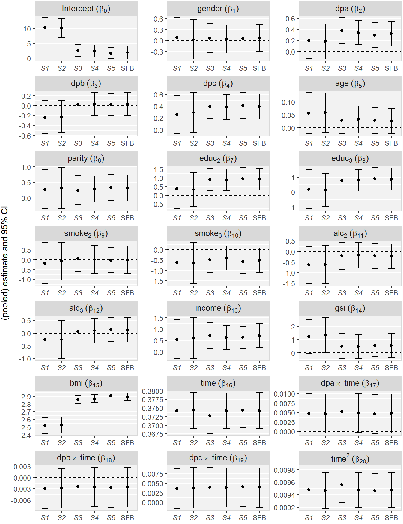
Figure 2.2: Parameter estimates and 95% CIs for the regression coefficients from the Generation R example for the five MICE strategies (S1 – S5) and the sequential fully Bayesian approach (SFB). The displayed CIs for SFB are the 2.5% and 97.5% quantiles of the MCMC sample.

Several coefficients demonstrate substantial differences in the estimates and CIs between different imputation strategies. Overall, MICE strategies S1 and S2 resulted in similar estimates and CIs, which however differed considerably from the estimates and/or CIs of the other three MICE strategies and the SFB approach, for most parameters. The naive MICE approaches S1 and S2 estimated non-significant effects for dpa, dpc and educ, whereas the other approaches estimated effects that were significantly different from zero. The largest difference between the strategies was observed for the parameter of bmi. The posterior mean and CIs for all regression coefficients are displayed in Table 2.2 in Appendix 2.B. These results indicate that, in the present example, a considerable amount of information is lost when the outcome is not represented by a summary of all its observations but only the first measurement or excluded completely from the imputation models in MICE.

2.5 Simulation Study

2.5.1 Design

To compare the performance of MICE and the SFB approach under different scenarios of missing data mechanisms, we performed a simulation study in which the missingness of the covariates depended on the outcome in different ways.

We simulated data for 500 subjects from a linear mixed-effects model \[ \begin{aligned} y_{ij} =& \beta_0 + \beta_1 \texttt{time}_{ij} + \beta_2 \texttt{time}_{ij}^2 + \beta_3 \texttt{B}_i + \beta_4 \texttt{C}_i + \beta_5 \texttt{C}_i\times\texttt{time}_{ij} +\\ & b_{i0} + \texttt{time}_{ij} b_{i1} + \texttt{time}_{ij}^2 b_{i2} + \varepsilon_{ij}, \end{aligned} \]

with \(j=1,\ldots,6\), a time variable that was uniformly distributed between 0 and 3.5, a binary cross-sectional covariate \(\texttt{B}_i\), creating two groups of equal size, a continuous cross-sectional covariate \(\texttt{C}_i\) that follows a standard normal distribution and is independent from \(\texttt{B}_i\), and error terms \(\varepsilon_{ij}\) from a normal distribution with mean zero and variance \(\sigma_y^2 = 0.25\). The random effects were assumed to be multivariate normal with mean \(\mathbf 0\) and covariance matrix \(\mathbf D\). The values of \(\boldsymbol\beta\) and \(\mathbf D\) that were used in each of the scenarios can be found in Appendix 2.C. To create an unbalanced design, repeated measurements were removed with probability 0.2 and under the restriction that each individual had to have at least three repeated measurements. The remaining time points were sorted for each subject.

In order to create missingness that depends on the longitudinal structure of the outcome, in Scenario 1 we obtained ordinary least squares estimates \(\boldsymbol{\hat \lambda}_i\) of the regression coefficients from preliminary linear models \[ \texttt{y}_{ij} = \lambda_{0i} + \lambda_{1i}\texttt{time}_{ij} + \lambda_{2i} \texttt{time}_{ij}^2 + \tilde{\varepsilon}_{ij}, \quad \tilde{\varepsilon}_{ij}\sim N(0, \sigma_\varepsilon^2), \] for each individual \(i\) and \(\texttt{C}_i\) was put to missing with probability \[ \mbox{logit}(p_i) = \gamma_0 + \gamma_1 \hat\lambda_{0i} + \gamma_2 \hat\lambda_{1i} + \gamma_3 \hat\lambda_{2i}, \] where \(\mbox{logit(x)} = \log\left\{x/(1-x)\right\}\). The values of \(\boldsymbol\gamma\) used for the simulation can be found in Table 2.4 in Appendix 2.C.

In Scenario 2, missing values were created in \(\texttt{B}_i\) as well as \(\texttt{C}_i\), depending on the area under the curve (AUC) described by the observed outcome \(\texttt{y}_{ij}\). The AUC for individual \(i\) was computed as \[ \mbox{AUC}_i = \sum_{j=1}^{n_i-1} (\texttt{time}_{ij+1}-\texttt{time}_{ij}) \frac{\texttt{y}_{ij} + \texttt{y}_{ij+1}}{2}, \] where \(n_i\) is the number of repeated measurements of individual \(i\), and scaled to be centred around zero and have standard deviation equal to 1, for computational reasons.

The probability \(p_{1i}\) of the continuous variable \(\texttt{C}_i\) to be missing was then computed as \[ \mbox{logit}(p_{1i}) = \gamma_{10} + \gamma_{11}\mbox{AUC}_i + \gamma_{12}\mbox{AUC}_i^2. \]

Observations in the binary variable \(\texttt{B}_i\) were deleted depending on the AUC and the missingness of \(\texttt{C}_i\) with probability \(p_{2i}\):

\[\mbox{logit}(p_{2i}) = \gamma_{20} + \gamma_{21}\unicode{x1D7D9}\;\,(\texttt{C}_i=\mbox{NA}) + \gamma_{22}\mbox{AUC}_i,\]

where \(\unicode{x1D7D9}\;\,\) is the indicator function which is 1 if \(\texttt{C}_i\) is missing and 0 otherwise.

In both scenarios, we performed the analysis based on the complete data as well as datasets with 20% and 50% missings. In Scenario 2, 60% of that desired missing percentage was missing in \(\texttt{C}_i\), the remaining 40% in \(\texttt{B}_i\). The coefficients \(\gamma_1, \gamma_2, \gamma_3, \gamma_{11}, \gamma_{12}, \gamma_{21}\) and \(\gamma_{22}\) were specified a priori and the intercepts \(\gamma_0, \gamma_{10}\) and \(\gamma_{20}\) chosen so that (approximately) the desired proportion of data was missing. All parameter values used for the simulation can be found in Appendix 2.C.

Under both scenarios, the simulated data were again imputed and fitted, using the correct analysis model, with the five strategies using MICE described in Section 2.4, as well as the SFB approach. Here, \(\texttt{time}_{i1}\) was included in strategy S2, strategy S4 used empirical Bayes estimates of the random intercept and slope and strategy S5 used estimates of the random intercept and the random effects for time and \(\texttt{time}^2\). We created 10 imputed datasets with each MICE strategy. In the SFB approach, we simulated three chains. The number of iterations was determined based on two criteria: the Gelman-Rubin criterion (Gelman, Meng, and Stern 1996) for convergence had to be smaller than 1.2 and the MCMC error less than five per cent of the parameter’s standard deviation (Lesaffre and Lawson 2012). An example of the JAGS syntax used for Scenario 2 can be found in Appendix 2.E.

It is important to note that S1 and S2 are not correct models under the MAR assumption in neither of the two scenarios since not all available information of \(\mathbf y_{i}\) and \(\texttt{time}_i\) is included.

2.5.2 Results

Under Scenario 1, the most severely biased estimates were observed for \(\beta_1\) (related to time) and \(\beta_5\) (related to the interaction between time and C). Figures 2.3 and 2.4 compare the relative bias (estimated \(\hat\beta\) divided by true \(\beta\)) and coverage rate of the 95% CIs, respectively, for all imputation strategies and missing percentages in Scenario 1.

Table 2.6 in Appendix 2.D summarizes the results from both simulation studies. For each covariate, the first line gives the average relative bias of the estimated parameter over all 500 simulations, the second line gives the mean squared error (MSE) of the estimates multiplied by ten and the third line gives the proportion of simulations in which the estimated 95% CI, or the 95% credible interval for the Bayesian analysis, covered the true \(\beta\).

MICE models S1 and S2 performed the worst, with a relative bias of 0.10 and 0.25 under 20% missing values, and a relative bias of -0.39 and -0.61 under 50% missing values. The coverage rate of the 95% CIs for both models was 20% and 30% respectively, under 20% missing values, and 5% and 0%, respectively, when only half of the individuals had \(\texttt{C}\) observed.

Summarizing \(\mathbf y_i\) by its mean (S3) resulted in less biased results (relative bias 0.82, 92% coverage under 20% missing values). For 50% missing values the relative bias worsened to 0.39 and the coverage rate dropped to 54%. S4 gave slightly biased estimates for the effect of time and the continuous covariate C and the CI of the parameter for C covered the true parameter only in 85.8% of the simulations under 50% missing values. S5 and the SFB approach were unbiased for all missing percentages and had only minor deviations from the desired coverage rate of 95%. The same difference between the imputation strategies was observed for the interaction between time and C, the intercept and the parameter of the continuous variable C, although less severe in the latter case. Again, S1 and S2 led to the most biased parameters and had (very) poor coverage rate, S3 was less biased and had insufficient coverage rate for the parameter of the interaction term. Also for these parameters, the SFB approach provided unbiased estimates with the desired coverage rate. The SFB approach had slightly smaller MSE than S4 and S5 for most parameters.

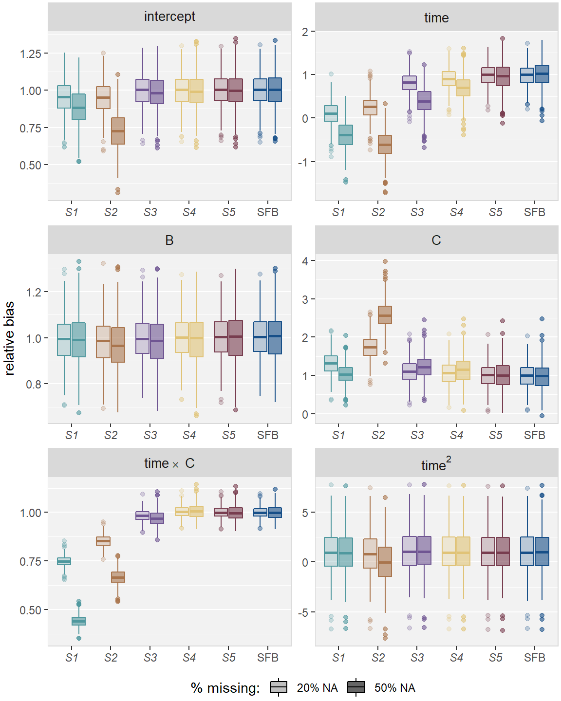
Figure 2.3: Relative bias in simulation , for the five imputation strategies using MICE (–) and the sequential fully Bayesian approach (SFB).

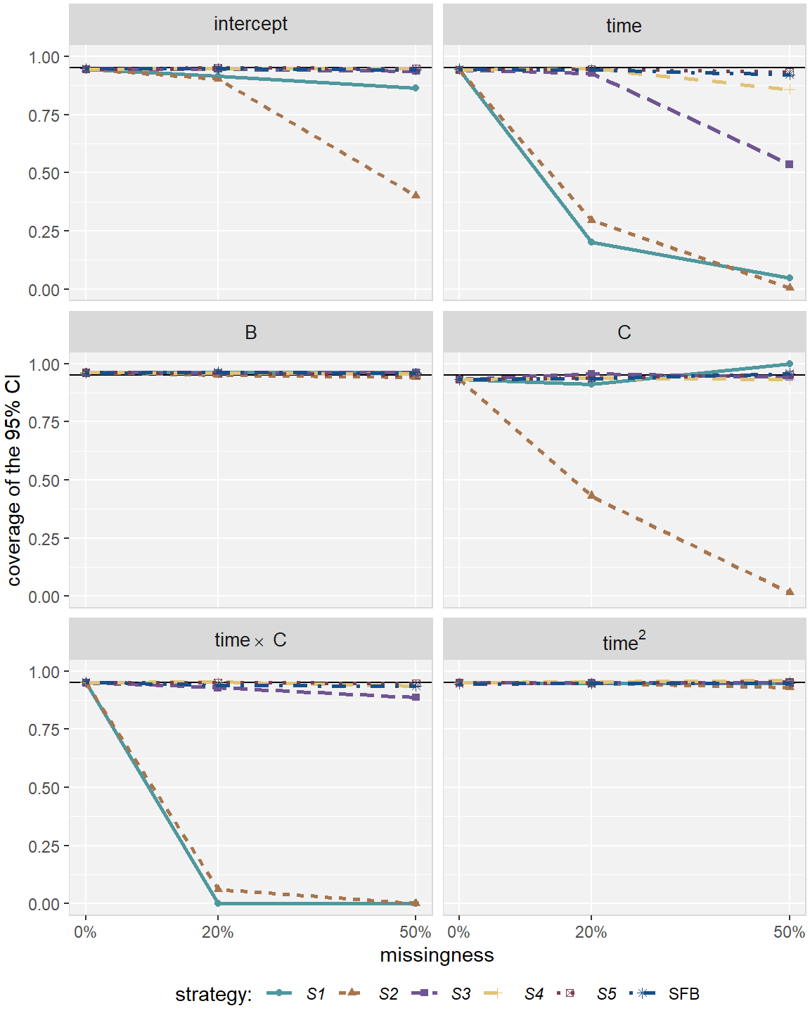
Figure 2.4: Coverage rate in simulation , for the five imputation strategies using MICE (–) and the sequential fully Bayesian approach (SFB).

In Scenario 2, S1 and S2 gave biased estimates and produced CIs with insufficient coverage rate for most parameters (see Figures 2.5 and 2.6 in Appendix 2.D). Estimates from S1 were more biased than those from S2 except for the parameter of the continuous covariate and time. S3 performed better than S1 and S2 for most parameters but still gave biased estimates and had coverage rate below 85% under 50% missing for the intercept and the effects for B and the interaction between B and time. The two more sophisticated MICE strategies S4 and S5, as well as the SFB approach, provided unbiased estimates and CIs with the desired coverage rate for all parameters.

The average computation time per simulation for the complete data was less than one second for lmer() and 15 seconds for the Bayesian model. For incomplete data, the computational time increased to 7 – 10 seconds for imputation with and subsequent analysis with lmer() and to 16 – 38 seconds for the SFB approach. The exact numbers can be found in Table 2.5 in Appendix 2.D.

2.6 Discussion

In this chapter, we have studied the statistical analysis of longitudinal outcomes with incomplete covariates. We have contrasted the popular MICE approach with a full specification of the joint distribution of the outcome and the covariates using the SFB approach. Our theoretical and simulation results suggest that the key in obtaining unbiased estimates is to sample the missing covariates from conditional distributions which are compatible with the other imputation models and with the analysis model of interest.

In MICE the full conditionals are specified directly and the outcome has to be included explicitly in the imputation models. When the outcome is multivariate and the covariates are of mixed type it is not straightforward to derive a functional form of the outcome to include in the corresponding linear predictors that would lead to compatible imputation models.

One way to ensure compatibility is to specify the joint distribution of all variables and derive the full conditionals from there. Bartlett et al. (2015) use a similar idea to extend MICE by proposing imputation using a “substantive model compatible full conditional specification”. Another approach (Carpenter and Kenward 2013; Goldstein et al. 2009) is to specify the joint distribution as (latent) multivariate normal and to draw multiple imputations from the resulting conditional distributions. The SFB approach uses a sequence of univariate conditional distributions to specify the joint distribution. This has the advantage that, since the analysis model is part of the conditional distributions, the parameters of interest are estimated simultaneously with the imputation of the missing values and no additional analysis (and pooling) is necessary. Furthermore, the specification of the univariate conditional imputation models allows for a straightforward and very flexible implementation.

The separation of the imputation and analysis step in MI is often considered an advantage because the set of completed datasets can be used for several analyses. The same is possible when data are imputed with the SFB approach: random draws from the posterior samples of the imputed values may be used to form multiple imputed datasets. However, the compatibility of the imputation models with the new analysis models cannot be guaranteed. If the analysis model changes considerably, the imputation has to be re-done. When using the SFB approach this may be time-consuming.

The possibility to include auxiliary variables, which are not part of the analysis model but are used to aid the imputation, is another attractive feature of MI. The SFB approach can be extended to include such auxiliary variables by including them in predictors of the imputation models but omitting them from the predictor of the analysis model or fixing the corresponding regression coefficients in the analysis model to zero. The implied assumption is therefore that the outcome is conditionally independent of the auxiliary variables.

A major reason why MICE is widely used is its availability in many software packages (Sterne et al. 2009; White, Royston, and Wood 2011; Yucel 2011). There are several packages in R that make use of the Bayesian framework for imputation (Quartagno and Carpenter 2015; Zhao and Schafer 2015; Van Buuren and Groothuis-Oudshoorn 2011; Bartlett 2015) but to our knowledge, none of them can currently handle missing baseline covariates of mixed types in a longitudinal setting. With the use of programs like WinBUGS (Lunn et al. 2000) or JAGS (Plummer 2003) however, the implementation and estimation of the SFB approach is straightforward (see example syntax in Appendix 2.E).

Even though it has been shown that MICE performs well in most standard situations and that the issue of incompatible imputation models is mainly a theoretical issue (Zhu and Raghunathan 2015), our results demonstrate the advantage of working with the full likelihood in more complex situations. This may as well be relevant when using other multivariate models, such as for instance latent mixture models, where imputation with MICE without taking into account the actual structure of the measurement model may lead to poorly imputed values which will distort the analysis. The SFB approach we presented in this chapter can be extended to such other multivariate outcomes in a straightforward and natural way and even allows for settings with multiple outcomes of possibly different types.

Appendix

2.A Variable Description

Table 2.1: Description of the covariates in the Generation R data.

name	description	level	missings
weight_0	maternal pre-pregnancy weight in kg	continuous	478	(14.2 %)
weight_1	maternal weight in first trimester in kg	continuous	550	(16.3 %)
weight_2	maternal weight in second trimester in kg	continuous	124	(3.7 %)
weight_3	maternal weight in third trimester in kg	continuous	99	(2.9 %)
dpa, dpb, dpc	dietary patterns (first three components from PCA)	continuous	–
gender	gender of the child (boys, girls)	binary	–
age	mother’s age at intake in years	continuous	–
height	mother’s height at intake in cm	continuous	1	(<0.1 %)
parity	previous births (none vs one or more)	binary	8	(0.2 %)
educ	gducational level of the mother (low and midlow, midhigh, high)	categorical	45	(1.3 %)
smoke	maternal smoking during pregnancy (never, until pregnancy was known continued during pregnancy)	categorical	250	(7.4 %)
alc	maternal alcohol intake during pregnancy (never, until pregnancy was known, continued during pregnancy)	categorical	272	(8.1 %)
income	monthly net household income (\(\leq\) 2200 €, >2200 €	binary	347	(10.28 %)
gsi	Global Severity Index (stress measure)	continuous	406	(12.0 %)
bmi	maternal BMI at intake (\(\frac{weight_0}{(height/100)^2}\))	continuous	478	(14.2 %)

2.B Results from the Generation R Data

Table 2.2: Pooled parameter estimates and 95% CIs or posterior means and 2.5% and 97.5% quantiles (SFB) of the analysis of the Generation R data. (S1: no outcome, S2: baseline outcome, S3: mean outcome, S4: simple random effects, S5: full random effects, SFB: sequential fully Bayesian)

2.C Simulation Settings

Table 2.3: Parameters \(\beta\) used for simulation.

	Intercept	time	B	C	time×B	time2
Scenario 1	0.97	0.36	1.4	0.25	2.46	0.01
Scenario 2	0.97	0.36	1.4	0.25	2.46	0.35

Table 2.4: Parameters \(\gamma\) used for simulation.

20% NA	50% NA	both
Scenario 1
\(\gamma_{0\phantom{0}} \approx\) -13.2	\(\gamma_{0\phantom{0}} \approx\) -6.9	\(\gamma_{1\phantom{1}}\) = 1.0	\(\gamma_{2\phantom{2}}\) = -3.5	\(\gamma_3 = 2.5\)
Scenario 2
\(\gamma_{10} \approx\) -2.8	\(\gamma_{10} \approx\) -1.2	\(\gamma_{11}\) = 2.5	\(\gamma_{12}\) = -0.5
\(\gamma_{20} \approx\) -3.0	\(\gamma_{20} \approx\) -2.1	\(\gamma_{21}\) = 1.5	\(\gamma_{22}\) = 0.5

\[D = \left(\begin{array}{rrr} 2.300 & -0.750 & -0.060 \\ -0.750 & 1.550 & 0.004 \\ -0.060 & 0.004 & 0.058 \\ \end{array}\right)\]

2.D Simulation Results

Table 2.5: Computational times in seconds for simulation in both scenarios.

	Scenario 1			Scenario 2
	0% NA	20% NA	50% NA	0% NA	20% NA	50% NA
S1	0.59	7.77	8.14	0.59	8.67	9.50
S2	0.59	6.89	7.44	0.59	8.62	8.85
S3	0.59	7.70	7.87	0.59	9.58	9.64
S4	0.59	6.82	6.87	0.59	8.72	8.72
S5	0.59	7.29	7.31	0.59	9.30	9.27
SFB	14.99	16.01	23.03	14.71	26.58	37.66

Table 2.6: Simulation results from both scenarios: relative bias, 10 times the mean squared error (MSE) and coverage rate of the 95% CI (S1: no outcome, S2: baseline outcome, S3: mean outcome, S4: simple random effects, S5: full random effects, SFB: sequential fully Bayesian)

		Scenario 1			Scenario 2
		rel. bias	10 × MSE	coverage	rel. bias	10 × MSE	coverage
full data
Intercept	lmer()	1.00	0.11	95%	1.00	0.11	95%
	SFB	1.00	0.11	95%	1.00	0.11	94%
time	lmer()	0.99	0.07	94%	0.99	0.07	94%
	SFB	0.99	0.07	95%	0.99	0.07	94%
B	lmer()	1.00	0.16	96%	1.00	0.16	96%
	SFB	1.00	0.16	96%	1.00	0.16	96%
C	lmer()	0.99	0.06	93%	0.99	0.06	93%
	SFB	0.99	0.06	93%	0.99	0.06	93%
time×B	lmer()	1.00	0.04	95%	1.00	0.04	95%
	SFB	1.00	0.04	95%	1.00	0.04	95%
time2	lmer()	1.04	0.00	95%	1.00	0.00	95%
	SFB	1.04	0.00	94%	1.00	0.00	95%
20% missing values
Intercept	S1	0.95	0.15	91%	1.11	0.24	87%
	S2	0.95	0.15	90%	1.04	0.14	94%
	S3	1.00	0.12	95%	1.05	0.14	94%
	S4	1.00	0.11	95%	1.00	0.12	96%
	S5	1.00	0.11	95%	1.00	0.12	95%
	SFB	1.00	0.12	95%	1.00	0.12	95%
time	S1	0.10	1.14	20%	1.33	0.22	82%
	S2	0.25	0.81	30%	1.17	0.12	91%
	S3	0.82	0.12	93%	1.00	0.07	95%
	S4	0.91	0.09	95%	0.99	0.07	94%
	S5	0.99	0.07	94%	1.00	0.07	95%
	SFB	0.99	0.07	94%	0.99	0.07	94%
B	S1	0.99	0.20	96%	0.88	0.46	87%
	S2	0.98	0.20	95%	0.96	0.21	95%
	S3	1.00	0.18	96%	0.93	0.27	93%
	S4	1.00	0.17	96%	1.00	0.18	96%
	S5	1.00	0.17	96%	1.00	0.18	95%
	SFB	1.00	0.17	96%	1.00	0.18	96%
C	S1	1.31	0.12	91%	0.92	0.06	97%
	S2	1.74	0.41	43%	1.16	0.08	92%
	S3	1.10	0.07	96%	1.00	0.06	96%
	S4	1.05	0.07	94%	1.00	0.06	93%
	S5	1.00	0.07	94%	0.99	0.06	95%
	SFB	0.99	0.07	94%	1.00	0.06	94%
time×B	S1	0.75	3.92	0%	0.91	0.53	45%
	S2	0.85	1.37	6%	0.95	0.19	78%
	S3	0.98	0.07	93%	0.99	0.05	94%
	S4	1.00	0.06	95%	1.00	0.05	95%
	S5	1.00	0.05	95%	1.00	0.05	95%
	SFB	1.00	0.05	94%	1.00	0.05	95%
time2	S1	1.01	0.00	95%	1.00	0.00	96%
	S2	0.84	0.00	95%	1.00	0.00	96%
	S3	1.10	0.00	95%	1.00	0.00	95%
	S4	1.03	0.00	95%	1.00	0.00	95%
	S5	1.04	0.00	95%	1.00	0.00	95%
	SFB	1.04	0.00	95%	1.00	0.00	95%
50% missing values
Intercept	S1	0.88	0.28	86%	1.28	0.85	42%
	S2	0.73	0.86	40%	1.12	0.28	84%
	S3	0.98	0.13	94%	1.14	0.31	82%
	S4	0.99	0.13	95%	1.01	0.14	95%
	S5	1.00	0.13	95%	1.00	0.14	94%
	SFB	1.00	0.13	94%	1.00	0.14	95%
time	S1	-0.39	2.65	5%	1.72	0.77	35%
	S2	-0.61	3.49	0%	1.41	0.30	75%
	S3	0.39	0.61	54%	1.01	0.08	95%
	S4	0.70	0.24	86%	0.98	0.07	94%
	S5	0.96	0.15	93%	0.99	0.07	94%
	SFB	1.01	0.13	92%	0.99	0.07	94%
B	S1	0.99	0.22	96%	0.69	2.05	32%
	S2	0.97	0.25	94%	0.89	0.47	88%
	S3	0.99	0.23	96%	0.81	0.91	69%
	S4	0.99	0.23	96%	0.98	0.25	95%
	S5	1.00	0.23	95%	1.00	0.25	94%
	SFB	1.00	0.20	96%	1.00	0.23	96%
C	S1	1.04	0.04	100%	0.80	0.08	95%
	S2	2.59	1.65	2%	1.41	0.18	82%
	S3	1.22	0.09	94%	1.05	0.07	96%
	S4	1.14	0.09	93%	1.03	0.07	94%
	S5	1.01	0.08	95%	1.00	0.07	94%
	SFB	0.97	0.08	96%	1.00	0.07	94%
time×B	S1	0.44	19.06	0%	0.78	2.93	0%
	S2	0.67	6.84	0%	0.87	1.00	13%
	S3	0.97	0.15	89%	0.98	0.08	90%
	S4	1.01	0.09	93%	0.99	0.05	95%
	S5	1.00	0.08	95%	1.00	0.05	95%
	SFB	1.00	0.08	94%	1.00	0.05	95%
time2	S1	0.97	0.00	95%	1.00	0.00	95%
	S2	0.02	0.01	93%	1.01	0.00	95%
	S3	1.12	0.00	95%	1.00	0.00	95%
	S4	1.02	0.00	96%	1.00	0.00	95%
	S5	1.02	0.00	95%	1.00	0.00	95%
	SFB	1.02	0.00	95%	1.00	0.00	94%

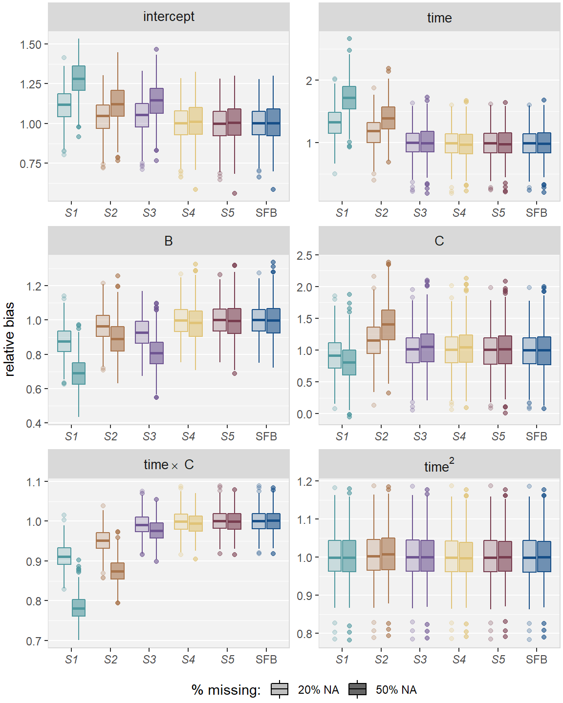
Figure 2.5: Relative bias in simulation Scenario 2, for the five imputation strategies using MICE (S1 – S5) and the sequential fully Bayesian approach (SFB).

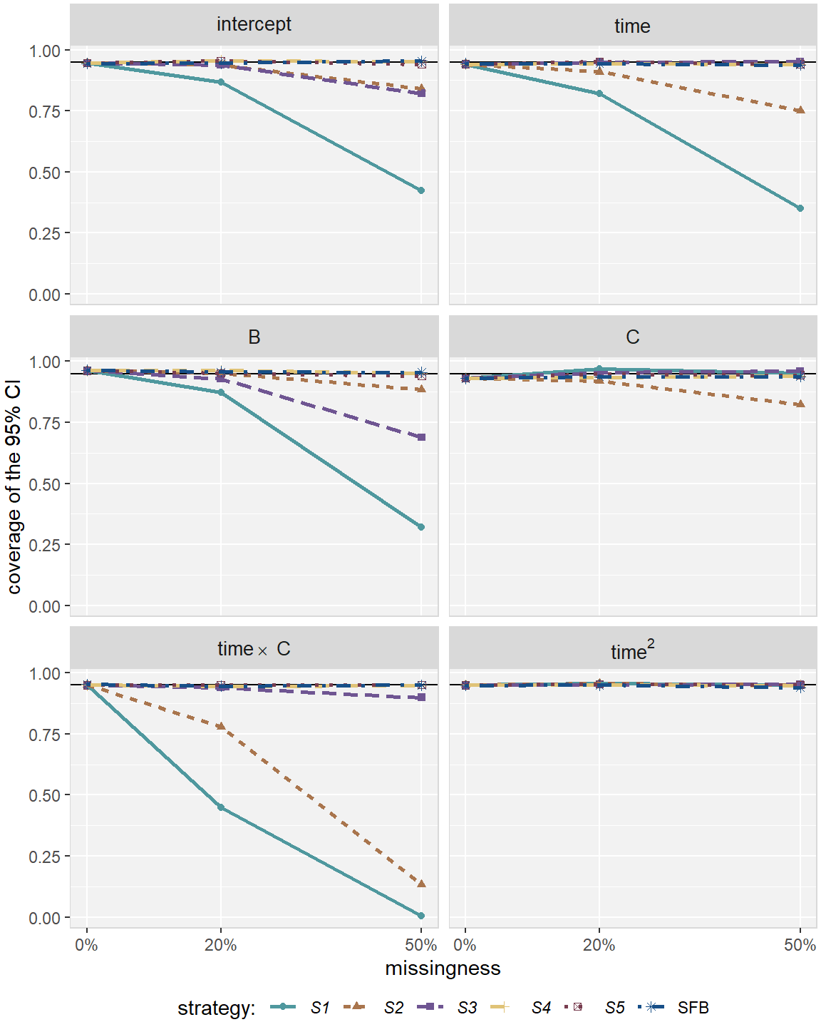
Figure 2.6: Coverage rate in simulation Scenario 2, for the five imputation strategies using MICE (S1 – S5) and the sequential fully Bayesian approach (SFB).

2.E JAGS Syntax for Simulation Scenario 2

It is convenient to implement the SFB approach using hierarchical centring. This means that the fixed effects enter the linear predictor through the random effects, i.e., the random effects are not centred around zero but around the fixed effects.

Data / Notation:

• TN: number of observations in the dataset
• N: number of individuals
• priorR: 3 \(\times\) 3 diagonal matrix of NA’s

model {
  for(j in 1:TN){
    # Linear mixed effects model for y
    y[j] ~ dnorm(mu.y[j], tau.y)
    mu.y[j] <- inprod(b[subj[j], ], Z[j, ]) # lin. predictor with
                                            # hierarchic. centring
                                            # specification
  }

  for(i in 1:N){
    b[i, 1:3] ~ dmnorm(mu.b[i, ], inv.D[ , ])
    mu.b[i, 1] <- beta[1] + beta[2] * B[i] + beta[3] * C[i]
    mu.b[i, 2] <- beta[4] + beta[5] * C[i]
    mu.b[i, 3] <- beta[6]
  }

  # Priors for analysis model: fixed effects
  for(k in 1:6){
    beta[k] ~ dnorm(0, 0.1)
  }
  tau.y ~ dgamma(0.001, 0.001)
  sigma.y <- sqrt(1/tau.y)

  # Priors for analysis model: random effects
  for(k in 1:3){
    priorR.invD[k,k] ~ dgamma(0.1, 0.01)
  }
  inv.D[1:3, 1:3] ~ dwish(priorR[, ], 3)
  D[1:3, 1:3] <- inverse(inv.D[, ])

  # imputation models
  for(i in 1:N){
    # normal regression for C
    C[i] ~ dnorm(mu.C[i], tau.C)
    mu.C[i] <- alpha[1]

    # binary regression for B
    B[i] ~ dbern(p.B[i])
    logit(p.B[i]) <- alpha[2] + alpha[3] * C[i]
  }

  # Priors for imputation of C
  for(k in 1:1){
    alpha[k] ~ dnorm(0, 0.001)
  }
  tau.C ~ dgamma(0.01, 0.01)

  # Priors for imputation of B
  for(k in 2:3){
    alpha[k] ~ dnorm(0, 4/9)
  }
}

References

Bartlett, Jonathan W. 2015. smcfcs: Multiple Imputation of Covariates by Substantive Model Compatible Fully Conditional Specification. http://CRAN.R-project.org/package=smcfcs.

Bartlett, Jonathan W., Shaun R. Seaman, Ian R. White, and James R. Carpenter. 2015. “Multiple Imputation of Covariates by Fully Conditional Specification: Accommodating the Substantive Model.” Statistical Methods in Medical Research 24 (4): 462–87. https://doi.org/10.1177/0962280214521348.

Bates, Douglas, Martin Mächler, Ben Bolker, and Steve Walker. 2015. “Fitting Linear Mixed-Effects Models Using lme4.” Journal of Statistical Software 67 (1): 1–48. https://doi.org/10.18637/jss.v067.i01.

Carpenter, James R., and Michael G. Kenward. 2013. Multiple Imputation and Its Application. John Wiley & Sons, Ltd. https://doi.org/10.1002/9781119942283.

Chen, Baojiang, Y. Yi Grace, and Richard J. Cook. 2010. “Weighted Generalized Estimating Functions for Longitudinal Response and Covariate Data That Are Missing at Random.” Journal of the American Statistical Association 105 (489): 336–53. https://doi.org/10.1198/jasa.2010.tm08551.

Chen, Baojiang, and Xiao-Hua Zhou. 2011. “Doubly Robust Estimates for Binary Longitudinal Data Analysis with Missing Response and Missing Covariates.” Biometrics 67 (3): 830–42. https://doi.org/10.1111/j.1541-0420.2010.01541.x.

Chen, Ming-Hui, and Joseph G. Ibrahim. 2001. “Maximum Likelihood Methods for Cure Rate Models with Missing Covariates.” Biometrics 57 (1): 43–52. https://doi.org/10.1111/j.0006-341X.2001.00043.x.

Donders, A. Rogier T., Geert J. M. G. van der Heijden, Theo Stijnen, and Karel G. M. Moons. 2006. “Review: A Gentle Introduction to Imputation of Missing Values.” Journal of Clinical Epidemiology 59 (10): 1087–91. https://doi.org/10.1016/j.jclinepi.2006.01.014.

Garrett, Elizabeth S., and Scott L. Zeger. 2000. “Latent Class Model Diagnosis.” Biometrics 56 (4): 1055–67. https://doi.org/10.1111/j.0006-341X.2000.01055.x.

Gelman, Andrew, Xiao-Li Meng, and Hal Stern. 1996. “Posterior Predictive Assessment of Model Fitness via Realized Discrepancies.” Statistica Sinica 6 (4): 733–60.

Goldstein, Harvey, James R. Carpenter, Michael G. Kenward, and Kate A. Levin. 2009. “Multilevel Models with Multivariate Mixed Response Types.” Statistical Modelling 9 (3): 173–97. https://doi.org/10.1177/1471082X0800900301.

Ibrahim, Joseph G., Ming-Hui Chen, and Stuart R. Lipsitz. 2002. “Bayesian Methods for Generalized Linear Models with Covariates Missing at Random.” Canadian Journal of Statistics 30 (1): 55–78. https://doi.org/10.2307/3315865.

Jaddoe, Vincent W. V., Cornelia M. van Duijn, Oscar H. Franco, Albert J. van der Heijden, Marinus H. van Ijzendoorn, Johan C. de Jongste, Aad van der Lugt, et al. 2012. “The Generation R Study: Design and Cohort Update 2012.” European Journal of Epidemiology 27 (9): 739–56. https://doi.org/10.1007/s10654-012-9735-1.

Janssen, Kristel J. M., A. Rogier T. Donders, Frank E. Harrell Jr, Yvonne Vergouwe, Qingxia Chen, Diederick E. Grobbee, and Karel G. M. Moons. 2010. “Missing Covariate Data in Medical Research: To Impute Is Better Than to Ignore.” Journal of Clinical Epidemiology 63 (7): 721–27. https://doi.org/10.1016/j.jclinepi.2009.12.008.

Knol, Mirjam J., Kristel J. M. Janssen, A. Rogier T. Donders, Antoine C. G. Egberts, E. Rob Heerdink, Diederick E. Grobbee, Karel G. M. Moons, and Mirjam I. Geerlings. 2010. “Unpredictable Bias When Using the Missing Indicator Method or Complete Case Analysis for Missing Confounder Values: An Empirical Example.” Journal of Clinical Epidemiology 63 (7): 728–36. https://doi.org/10.1016/j.jclinepi.2009.08.028.

Lesaffre, Emmanuel M. E. H., and Andrew B. Lawson. 2012. Bayesian Biostatistics. John Wiley & Sons. https://doi.org/10.1002/9781119942412.

Little, Roderick J. A., and Donald B. Rubin. 2002. Statistical Analysis with Missing Data. Hoboken, New Jersey: John Wiley & Sons, Inc. https://doi.org/10.1002/9781119013563.

Lunn, David J., Andrew Thomas, Nicky Best, and David Spiegelhalter. 2000. “WinBUGS – a Bayesian modelling framework: Concepts, structure, and extensibility.” Statistics and Computing 10 (4): 325–37. https://doi.org/10.1023/A:1008929526011.

Molenberghs, Geert, and Michael G. Kenward. 2007. Missing Data in Clinical Studies. Statistics in Practice. Wiley. https://doi.org/10.1002/9780470510445.

Moons, Karel G. M., Rogier A. R. T. Donders, Theo Stijnen, and Frank E. Harrell Jr. 2006. “Using the Outcome for Imputation of Missing Predictor Values Was Preferred.” Journal of Clinical Epidemiology 59 (10): 1092–1101. https://doi.org/10.1016/j.jclinepi.2006.01.009.

Plummer, M. 2003. “JAGS: A Program for Analysis of Bayesian Graphical Models Using Gibbs Sampling.” Edited by Kurt Hornik, Friedrich Leisch, and Achim Zeileis.

Quartagno, Matteo, and James R. Carpenter. 2015. jomo: A Package for Multilevel Joint Modelling Multiple Imputation. http://CRAN.R-project.org/package=jomo.

R Core Team. 2013. R: A Language and Environment for Statistical Computing. Vienna, Austria: R Foundation for Statistical Computing. http://www.R-project.org/.

Rubin, Donald B. 1987. Multiple Imputation for Nonresponse in Surveys. Wiley Series in Probability and Statistics. Wiley. https://doi.org/10.1002/9780470316696.

Schafer, Joseph L. 1997. Analysis of Incomplete Multivariate Data. Chapman & Hall/Crc Monographs on Statistics & Applied Probability. Taylor & Francis.

Seaman, Shaun R., John Galati, Dan Jackson, and John Carlin. 2013. “What Is Meant by ‘Missing at Random’?” Statistical Science 28 (2): 257–68. https://doi.org/10.1214/13-STS415.

Sterne, Jonathan A. C., Ian R. White, John B. Carlin, Michael Spratt, Patrick Royston, Michael G. Kenward, Angela M. Wood, and James R. Carpenter. 2009. “Multiple Imputation for Missing Data in Epidemiological and Clinical Research: Potential and Pitfalls.” BMJ: British Medical Journal 338. https://doi.org/10.1136/bmj.b2393.

Stubbendick, Amy L., and Joseph G. Ibrahim. 2003. “Maximum Likelihood Methods for Nonignorable Missing Responses and Covariates in Random Effects Models.” Biometrics 59 (4): 1140–50. https://doi.org/10.1111/j.0006-341X.2003.00131.x.

Van Buuren, Stef. 2012. Flexible Imputation of Missing Data. Chapman & Hall/CRC Interdisciplinary Statistics. Taylor & Francis.

Van Buuren, Stef, and Karin Groothuis-Oudshoorn. 2011. “mice: Multivariate Imputation by Chained Equations in R.” Journal of Statistical Software 45 (3): 1–67. https://doi.org/10.18637/jss.v045.i03.

White, Ian R., Patrick Royston, and Angela M. Wood. 2011. “Multiple imputation using chained equations: Issues and guidance for practice.” Statistics in Medicine 30 (4): 377–99. https://doi.org/10.1002/sim.4067.

Yucel, Recai M. 2011. “State of the Multiple Imputation Software.” Journal of Statistical Software 45 (1). https://doi.org/10.18637/jss.v045.i01.

Zhao, Jing Hua, and Joseph L. Schafer. 2015. Pan: Multiple Imputation for Multivariate Panel or Clustered Data. https://CRAN.R-project.org/package=pan.

Zhu, Jian, and Trivellore E. Raghunathan. 2015. “Convergence Properties of a Sequential Regression Multiple Imputation Algorithm.” Journal of the American Statistical Association 110 (511): 1112–24. https://doi.org/10.1080/01621459.2014.948117.