Chapter 5 Bayesian Imputation of Time-varying Covariates in Mixed Models
This chapter is based on
Nicole S. Erler, Dimitris Rizopoulos, Vincent W. V. Jaddoe, Oscar H. Franco and Emmanuel M. E. H. Lesaffre. Bayesian imputation of time-varying covariates in linear mixed models. Statistical Methods in Medical Research, 2019; 28(2), 555 – 568. doi:10.1177/0962280217730851
Abstract
Studies involving large observational datasets commonly face the challenge of dealing with multiple missing values. The most popular approach to overcome this challenge, multiple imputation using chained equations, however, has been shown to be sub-optimal in complex settings, specifically in settings with longitudinal outcomes, which cannot be easily and adequately included in the imputation models. Bayesian methods avoid this difficulty by specification of a joint distribution and thus offer an alternative. A popular choice for that joint distribution is the multivariate normal distribution. In more complicated settings, as in our two motivating examples that involve time-varying covariates, additional issues require consideration: the endo- or exogeneity of the covariate and its functional relation with the outcome. In such situations, the implied assumptions of standard methods may be violated, resulting in bias. In this work, we extend and study a more flexible, Bayesian, alternative to the multivariate normal approach, to better handle complex incomplete longitudinal data. We discuss and compare assumptions of the two Bayesian approaches about the endo- or exogeneity of the covariates and the functional form of the association with the outcome, and illustrate and evaluate consequences of violations of those assumptions using simulation studies and two real data examples.
5.1 Introduction
Missing values are a common challenge in the analysis of observational data, especially in longitudinal studies.
This work is motivated by two research questions from the Generation R Study (Kooijman et al. 2016), a large longitudinal cohort study from fetal life onward. Specifically, the questions are: 1) “How is gestational weight associated with maternal blood pressure during pregnancy?”, and 2) “How is gestational weight associated with body mass index of the offspring during the first years of life?”. Due to the observational nature of the study, there is a considerable amount of incomplete data, with the particular challenge that missing values do not only occur in the outcome but also in baseline and time-varying covariates.
There are several well-established approaches to deal with incomplete data, the most popular being multiple imputation using chained equations (MICE) (Van Buuren 2012), which are readily available in standard statistical software. MICE has been shown to work well in many standard settings but may not be optimal in more complex applications, especially with longitudinal or other multivariate outcomes, which cannot be easily included in the imputation models for incomplete covariates in an appropriate manner (Erler et al. 2016). Fully Bayesian approaches provide a useful alternative in such complex settings, due to their ability to jointly model multivariate outcomes and incomplete covariates. The most popular omnibus approach in the Bayesian framework postulates a full multivariate normal distribution (Carpenter and Kenward 2013). Although this approach, as well as other approaches, is targeted towards a broad range of applications, in complex settings such as our two motivating research questions, the nature of the data requires careful consideration of the appropriateness of such standard methods and a more dedicated approach may be necessary. Especially with time-varying covariates, imputation and analysis become more demanding and, in order to obtain valid results, require additional considerations about the association between the time-varying covariates and the outcome. Specifically, endogenous covariates, i.e., covariates that are influenced by the outcome, and covariates that have non-standard functional relations with the outcome, can pose challenges that may or may not be adequately handled by standard methods, which usually assume linear associations and implicitly assume exogeneity of the covariates.
In the present paper, we focus on two approaches in the Bayesian framework to deal with covariates that are missing at random. The first approach is described by Carpenter and Kenward (2013). The basic idea is to assume a (latent) normal distribution for each incomplete variable and to connect them in such a way that the joint distribution is multivariate normal, which allows straightforward sampling to impute missing values. This approach is a common strategy to implement multiple imputation in longitudinal settings, where it can be used as the data generating step. The resulting data are then analysed in a second step with a complete data method, not necessarily Bayesian. While the multivariate normality assumption creates a convenient standardized framework, it thereby also implies linear relations between the variables involved, which may not be the case.
The second approach factorizes the joint distribution of the data into a sequence of conditional distributions, where the first conditional distribution can conveniently be chosen to be the analysis model of interest, allowing simultaneous imputation and analysis within the same procedure. This approach has been described previously for time-constant covariates (Erler et al. 2016) and we will extend it in the present paper to handle exogenous as well as endogenous time-varying covariates. The specification of separate models for each incomplete covariate requires somewhat more consideration than the specification of a multivariate normal distribution but makes this approach more flexible as well as capable of handling non-linear relationships. We will elucidate the capabilities and limitations of the two approaches with regards to different functional forms for, as well as endo- or exogeneity of, time-varying covariates and demonstrate how the use of an ‘off the shelf’ approach may be problematic in settings that require a more tailored approach.
The remainder of this chapter is structured as follows. We start with introducing the motivating dataset and describe in more detail the two research questions from the Generation R Study. In Section 5.3 we specify the linear mixed model for time-varying covariates and explore different functional forms as well as the issue of endo- and exogeneity. The two methods of interest are introduced in Section 5.4, where we will also discuss their implied assumptions about endo- or exogeneity of the covariates and their ability to handle different functional forms. We return to the Generation R data in Section 5.5, where we demonstrate how the two methods under investigation can be applied. A more formal evaluation of the methods follows in Section 5.6 where we perform a simulation study. Section 5.7 concludes this paper with a discussion.
5.2 Generation R Data
The Generation R Study is a population-based prospective cohort study from early fetal life onward, conducted in Rotterdam, the Netherlands (Kooijman et al. 2016). An important field of research within the Generation R Study is the exploration of how the mother’s condition during pregnancy may affect her own health and that of her child. Especially weight gain during gestation is of interest as it is closely related to the development of the fetus, as well as to pregnancy comorbidities, such as gestational hypertension, that may adversely affect both mother and child (e.g., Tielemans et al. (2015)). Children’s growth and body composition, as for instance measured by BMI, is an important determinant of health throughout childhood and later life. Therefore, current research is concerned with the two questions stated in Section 5.1, i.e., the associations between maternal weight (gain) during pregnancy with maternal blood pressure during pregnancy as well as with child BMI after birth.
To investigate these two research questions, a subset of variables was
extracted from the Generation R Study. The dataset contains information on
7643 mothers who had singleton, live births no earlier than
37 weeks of gestation, and their children. Each woman was asked for her
pre-pregnancy weight (baseline) and to visit the research centre once in each
trimester, during which the weight (gw) was measured and the blood pressure
taken.
Since women were eligible to enter the study at any gestational age, prenatal
measurements for the first and second trimester are missing for women
who enrolled later in pregnancy. Furthermore, there is some intermittent missingness
in the gestational and blood pressure data.
There were 3515 women for whom all four weight measurements were
recorded, 3094 for whom three weight measurements were observed,
859 women had two measurements, and 175 women had
only one measurement of weight.
The gestational age at each measurement (gage) was recorded and the time point
of the baseline measurement was set to be zero for all women.
Systolic blood pressure (bp) was measured three times in 4755
women, 2403 women had only two measurements of blood pressure and
477 women just one measurement. For 8 women no
blood pressures were recorded.
Child BMI was measured up to 12 times
between the ages of
2 weeks and
5 years, with a median of
7 observations per child;
1848 children had no BMI measurements.
The child’s age in months (age) was recorded at each BMI measurement and age
and sex adjusted standard deviation scores were calculated (bmi).
A graphical summary of the missingness pattern of the gestational weight and
systolic blood pressure measurements, and the available child BMI measurements
is given in Figures 5.4 – 5.6 in
Appendix 5.B.
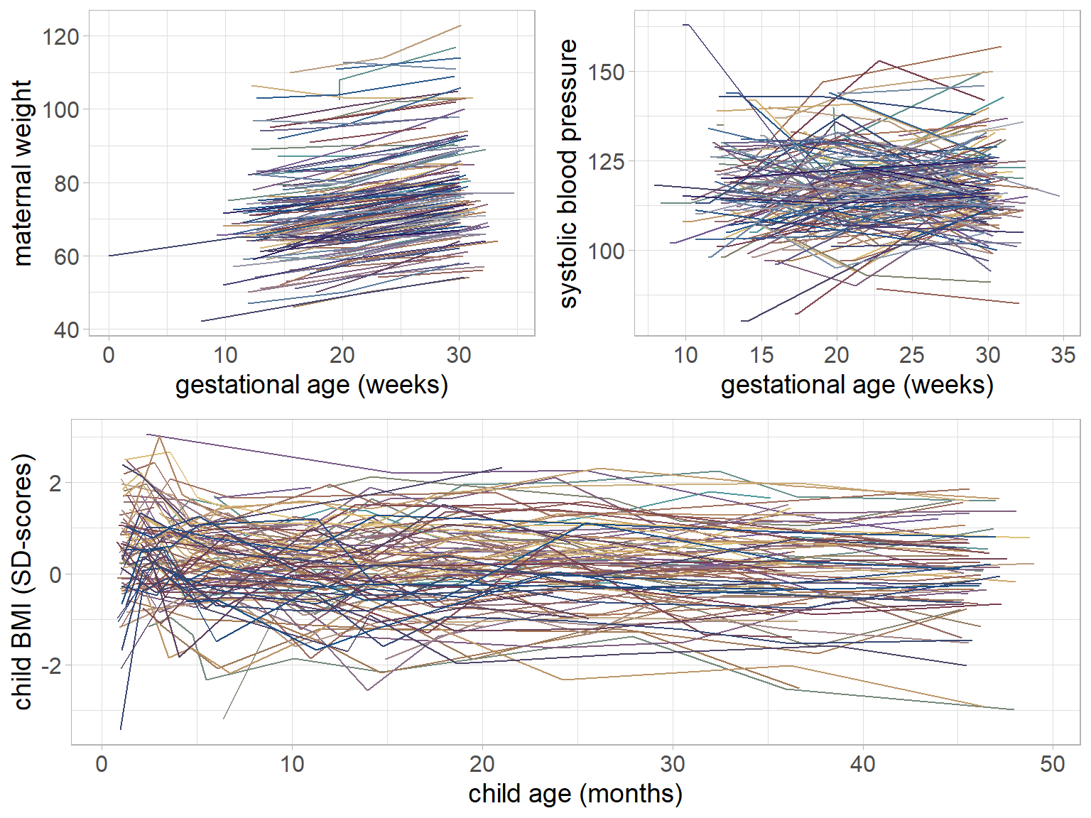
Figure 5.1: Trajectories of maternal weight, maternal systolic blood pressure and child BMI for a random sample of mothers and children from the Generation R data.
The trajectories of gw, bp and bmi of a random subset of individuals are
visualized in Figure 5.1.
Furthermore, we considered a number of potential confounders:
maternal age at intake (agem, continuous, complete),
maternal height (height, continuous,
0.38% missing values),
parity (parity, binary: nulliparous vs multiparous,
1.27% missing values),
maternal ethnicity (ethn, binary: European vs other,
5.59% missing values),
maternal education (educ, three ordered categories,
9.29% missing values)
and
maternal smoking habit during pregnancy (smoke, three ordered categories,
12.17% missing values).
Maternal BMI (bmim) was calculated as gestational weight (kg),
measured at time zero, divided by squared height (in m).
Logistic regression of the complete cases showed that
missingness in the baseline covariates (except for parity) was
associated with some or all of the other baseline covariates.
This indicates that missing values are not completely at random.
However, since this study was conducted in the general population subjects are
relatively healthy and the practical settings are such that it is reasonable
to believe that missing values in the clinical measurements, as for instance
gw or bmi, are at random, given the other variables.
It could be argued that missing values in the lifestyle variables,
especially in smoke, are not missing at random because mothers who are smoking
might be more inclined not to report it. If this was the case, the
mechanism that led to the missing values had to be included in the imputation
procedure since otherwise results would be biased. However, the assumption of
randomly missing data is untestable, and the missing data mechanism is usually
unknown, necessitating extensive sensitivity analysis.
As this exceeds the purpose of this study, we will
focus here on randomly missing data.
To make the assumption of randomly missing data more plausible, a number
of covariates will be considered in the analysis model, since omission of
relevant predictor variables may be another reason of not randomly missing data.
5.3 Modelling Longitudinal Data with Time-varying Covariates
5.3.1 Framework
A standard modelling framework for studying the relation between a longitudinal outcome and predictor variables is mixed effects modelling. As in our motivating case studies, often some of these predictors are time-varying. To facilitate exposition and also for notational simplicity in the following we only consider a single time-varying covariate. In particular, for a continuous longitudinal outcome we postulate the following mixed model \[ y_i(t) = \mathbf x_i(t)^\top\boldsymbol\beta + f(H^s_i(t), t)^\top \boldsymbol\gamma + \mathbf z_i(t)^\top\mathbf b_i + \varepsilon_i(t), \] where \(y_i(t)\) is the observation of individual \(i\) measured at time \(t\), \(\boldsymbol\beta\) denotes the vector of regression coefficients of the design matrix of the fixed effects \(\mathbf X_i\), with \(\mathbf x_{i}(t)\) being a column vector containing a row of that matrix, \(\mathbf z_i(t)\), a column vector expressing a row of the design matrix \(\mathbf Z_i\) of the random effects \(\mathbf b_i\sim N(\mathbf 0, \mathbf D)\), \(\boldsymbol\gamma\) is a vector of regression coefficients related to the time-varying covariate \(\mathbf s_i\), and \(\varepsilon_i(t)\sim N(0, \sigma_y^2)\) is an error term. Except for time itself, \(\mathbf X\) does not contain any time-varying covariates. To include \(\mathbf s\) in the linear predictor of \(\mathbf y\) assumptions about the relation between the two variables have to be made. These assumptions can be expressed by specifying a function \(f(H_i^s(t), t)\) which links the history of the time-varying predictor up to time \(t\), \(H_i^s(t) = \left\{s_i(t_{ij}): 0\leq t_{ij}\leq t, \; j=1,\ldots,n_i^s\right\}\), to the outcome, where \(t_{ij}\) is the time of the \(j\)-th measurement of individual \(i\) and \(n_i^s\) is the number of measurements of \(\mathbf s\) for that individual.
5.3.2 Functional Forms for Time-varying Covariates
The choice of an appropriate functional form implies that the following two questions need to be addressed. Namely, how are \(\mathbf s_i\) and \(\mathbf y_i\) related with regards to their time scales, and which features of \(\mathbf s_i\) are of interest in the relation with \(\mathbf y_i\)? The first question asks whether \(\mathbf y_i\) and \(\mathbf s_i\) have been measured in the same time intervals and whether their time scales have the same origin and unit. To allow for settings where \(\mathbf y_i\) and \(\mathbf s_i\) have been measured on different time scales, for instance maternal weight during pregnancy and child BMI after birth, we use \(t\) to denote the time scale of \(\mathbf y_i\) and \(\tilde t\) to denote the time scale of \(\mathbf s_i\). The second question relates to the specific application and is reflected in the choice of \(f(\cdot)\). Choices, that represent relevant features of gestational weight in our two motivating research questions are \[\begin{eqnarray} f(H_i^s(t), t) &=& s_i(t), \tag{5.1}\\ f(H_i^s(t), t) &=& \left\{\Delta_1(\mathbf s_i), \Delta_2(\mathbf s_i), \Delta_3(\mathbf s_i)\right\}^\top, \tag{5.2} \end{eqnarray}\]
with \[\begin{eqnarray*} \Delta_1(\mathbf s_i) &=& s_i(\tilde t_1) - s_i(\tilde t_0),\\ \Delta_2(\mathbf s_i) &=& s_i(\tilde t_2) - s_i(\tilde t_1),\\ \Delta_3(\mathbf s_i) &=& s_i(\tilde t_3) - s_i(\tilde t_2), \end{eqnarray*}\] where (5.1) represents the commonly chosen linear relation between the value of \(\mathbf s_i\), e.g., maternal weight, and \(\mathbf y_i\), e.g., blood pressure, measured at the same time points (i.e., \(t = \tilde t\)). Function (5.2) represents trimester specific weight gain, i.e., the difference of maternal weight over three given time intervals. In a more general notation, (5.1) could be written as \(f(H_i^s(t), t) = s_i(g(t))\) and refer to the value of \(\mathbf s_i\) at a time point that is specified by a function \(g(t)\), and (5.2) could be written as \(f(H_i^s(t), t) = s_i(g_2(t)) - s_i(g_1(t))\), where the time intervals are specified by the functions \(g_1(t)\) and \(g_2(t)\) and may not be the same for all \(t\).
In other applications, it is likely that different functional forms will be more appropriate. Such functions may, for instance, represent cumulative effects or use estimates of random effects associated with the individual profiles of the time-varying covariate. In cases where there is not a specific functional form of interest or there is uncertainty about which functional form is most appropriate, multiple functional forms can be included and shrinkage priors used to reduce correlations between parameters or to select the best suited functional form (Andrinopoulou and Rizopoulos 2016).
5.3.3 Endo- and Exogeneity
Another characteristic of the relation between a time-varying covariate and the outcome that needs to be considered is whether the time-varying covariate is exogenous or endogenous. Formally, exogeneity is defined by the following two conditions (Engle, Hendry, and Richard 1983; Diggle et al. 2002) \[ \left\{\begin{array}{l} \begin{align*} p(y_i(t), f(H^s_i(t), t) \mid H^y_i(t^-), H^s_i(t^-), \boldsymbol\theta) = & p(y_i(t) \mid f(H^s_i(t), t), H^y_i(t^-), H^s_i(t^-), \boldsymbol\theta_1) \times\\ & p(s_i(t) \mid H^y_i(t^-), H^s_i(t^-), \boldsymbol\theta_2)\\[2ex] p(s_i(t) \mid H^s_i(t^-), H^y_i(t^-), \mathbf x_i, \boldsymbol\theta) = & p(s_i(t) \mid H^s_i(t^-), \mathbf x_i, \boldsymbol\theta) \end{align*} \end{array} \right. \] where \(\boldsymbol\theta\) is a vector of parameters and other unknown quantities, with \(\boldsymbol \theta^\top = (\boldsymbol\theta_1^\top, \boldsymbol \theta_2^\top)\) and \(\boldsymbol\theta_1 \perp\!\!\!\perp \boldsymbol\theta_2\), and where \(H^y_i(t^-)\) and \(H^s_i(t^-)\) denote the history of \(\mathbf y\) and \(\mathbf s\), respectively, up to, but excluding measurements at time \(t\). By specifying the functional relation between \(\mathbf y_i\) and \(\mathbf s_i\) to be a function of the history of \(\mathbf s\), we avoid dependence of \(y_i(t)\) on future values of \(\mathbf s_i\), which is an additional requirement for exogeneity, see Diggle et al. (2002). Variables, for which these conditions are not satisfied are called endogenous. This may be the case for maternal weight as a predictor variable for blood pressure. Since both variables are measured in the same individual they may be subject to the same unmeasured influences or causal pathways may be reversed, which often entails endogeneity. In the setting where maternal weight is considered as a predictor of child BMI, however, the assumption of exogeneity may be more likely, since the covariate is measured earlier than the outcome and in different subjects.
Most common methods for inference, like generalized linear (mixed) regression models, assume covariates to be exogenous. If that assumption is wrong and the covariate is, in fact, endogenous, estimates may be biased (Diggle et al. 2002; Daniels and Hogan 2008).
5.4 Bayesian Analysis with Incomplete Covariates
As introduced in Section 5.2, the motivating questions from the Generation R Study involve outcomes and covariates that are incomplete. This holds for both the baseline and time-varying covariates. Hence, to appropriately investigate the associations of interest we need to account for missingness. In the Bayesian framework, missing values, whether they are in the outcome or in covariates, can be imputed in a natural and elegant manner. A common assumption, which we make here for the outcome as well as the covariates, is that the missing data mechanism is Missing At Random (MAR), i.e., the probability of a value being unobserved may depend on other observed values but not on values that have not been observed. In addition, the parameters of the analysis model are assumed to be independent of the missingness process. Under these assumptions, the missingness process is ignorable and does not need to be modelled (Little and Rubin 2002). Furthermore, this assumption entails that explicit imputation of the outcome is not necessary to obtain valid results, and we will, therefore, focus on settings with incomplete covariates. In this section, we adapt and implement two popular Bayesian approaches for analysing data with incomplete covariates, namely, the sequential approach (Ibrahim, Chen, and Lipsitz 2002; Erler et al. 2016), and the multivariate normal approach (Carpenter and Kenward 2013). In particular, we extend the first approach to settings with time-varying covariates that may be exogenous or endogenous. Both approaches model the joint distribution of the complete data and draw imputations from the posterior full conditional distributions that result from it but differ in the way the joint complete data distribution is specified. These differences influence how the two approaches can handle different functional forms as well as exo- versus endogenous covariates.
We start with some additional notation. As in the motivating data, the time-varying covariate \(\mathbf s\) is assumed to be incomplete. Missing values in \(\mathbf s\) occur not only due to missed measurements or drop-out but can also be caused when the functional form \(f(H_i^s(t), t)\) depends on values of \(\mathbf s\) that have not been (scheduled to be) measured. We use \(\mathbf s_i = (\mathbf s_{i, obs}^\top, \mathbf s_{i, mis}^\top)^\top\) to distinguish between the observed and missing values of \(\mathbf s\) for individual \(i\). Analogously, we assume two parts for the baseline covariates \(\mathbf X\) on the individual level: \(\mathbf x_{i,obs}\) and \(\mathbf x_{i, mis}\), which contain the observed and missing values of \(\mathbf x_i\), respectively. Furthermore, we use the partition \(\mathbf X = (\mathbf X_c, \mathbf x_1, \ldots, \mathbf x_p)\), where \(\mathbf X_c\) denotes the subset of covariates that are completely observed for all individuals, and \(\mathbf x_1, \ldots, \mathbf x_p\) are \(n\times 1\) vectors of those covariates that contain missing values.
5.4.1 Sequential Approach
The sequential approach to impute missing baseline covariates in models with longitudinal outcomes was previously presented by Erler et al. (2016) and will be extended here to incomplete time-varying covariates.
In our setting, the posterior distribution of interest (and associated joint distribution) is \[\begin{eqnarray*} p(\mathbf s_{mis}, \mathbf X_{mis}, \mathbf b, \boldsymbol\theta \mid \mathbf y, \mathbf s_{obs}, \mathbf X_{obs}) &\propto& p(\mathbf y, \mathbf s_{obs}, \mathbf X_{obs} \mid \mathbf s_{mis}, \mathbf X_{mis}, \mathbf b, \boldsymbol\theta)\\ && p(\mathbf s_{mis}, \mathbf X_{mis}, \mathbf b, \boldsymbol\theta)\\ & = & p(\mathbf y, \mathbf s_{obs}, \mathbf s_{mis}, \mathbf X_{obs}, \mathbf X_{mis}, \mathbf b, \boldsymbol\theta), \end{eqnarray*}\] where \(\boldsymbol\theta\) is a vector of unknown parameters, and can be factorized as \[\begin{equation} p(\mathbf y \mid \mathbf s, \mathbf X, \mathbf b, \boldsymbol\theta)\; p(\mathbf s \mid \mathbf X, \mathbf b, \boldsymbol\theta)\; p(\mathbf X \mid \boldsymbol\theta)\; p(\mathbf b \mid \boldsymbol\theta)\; p(\boldsymbol\theta), \tag{5.3} \end{equation}\] for which all terms can be specified based on known distributions.
The first term in (5.3), i.e., \(p(\mathbf y \mid \mathbf s, \mathbf X, \mathbf b, \boldsymbol\theta)\), is conveniently chosen to be the analysis model of interest, \[\begin{equation} y_i(t) = \mathbf x_i(t)^\top \boldsymbol\beta_{y\mid s,x} + f(H_i^s(t), t)^\top \boldsymbol\gamma + \mathbf z_i^y(t)^\top\mathbf b_i^y + \varepsilon_i^y(t), \tag{5.4} \end{equation}\] with random effects \(\mathbf b_i^y\sim N(0,\mathbf D_y)\) and \(\boldsymbol\varepsilon_i^y(t) \sim N(0, \sigma_y^2)\), and the second factor, representing the imputation model for the time-varying covariate, can be specified analogously as a linear mixed model \[\begin{equation} s_i(\tilde t) = \mathbf x_i(\tilde t)^\top \boldsymbol\beta_{s\mid x} + \mathbf z_i^s(\tilde t)^\top\mathbf b_i^s + \varepsilon_i^s(\tilde t), \tag{5.5} \end{equation}\] with \(\mathbf b_i^s\sim N(0,\mathbf D_s)\) and \(\boldsymbol\varepsilon_i^s(\tilde t) \sim N(0, \sigma_s^2)\). All variance matrices \(\mathbf D\) and parameters \(\sigma^2\) are assumed to follow vague inverse-Wishart and inverse-gamma distributions, respectively. Inclusion of \(f(H_i^s(t), t)\) in the linear predictor for \(\mathbf y_i\) allows for a large variety of possibly non-linear relations between \(\mathbf y_i\) and \(\mathbf s_i\), also when they are measured on different time scales. The joint distribution of the baseline covariates \(\mathbf X\) is often a multivariate distribution of mixed type variables for which usually no closed form solution is known. It can, however, be specified as a sequence of univariate conditional distributions (Ibrahim, Chen, and Lipsitz 2002; Erler et al. 2016), \(\boldsymbol\theta_x^\top = (\boldsymbol\theta_{x_1}^\top, \ldots, \boldsymbol\theta_{x_p}^\top)\), where \(\mathbf x_\ell\) denotes the \(\ell\)-th incomplete covariate. The univariate conditional distributions are assumed to be members of the exponential family, extended with distributions for ordinal categorical variables, with linear predictors \[\begin{eqnarray*} g_\ell\left\{E\left(\mathbf x_\ell \mid \mathbf X_c, \mathbf x_1, \ldots, \mathbf x_{\ell-1}, \boldsymbol\theta_{x_\ell}\right)\right\} &=& \mathbf X_c \boldsymbol\alpha_{\ell} + \sum_{q = 1}^{\ell - 1} \mathbf x_q \xi_{\ell_q}, \end{eqnarray*}\] which allows an easy and flexible specification in settings with many covariates of mixed type, since each link function \(g_\ell\) can be chosen separately and appropriately for \(\mathbf x_\ell\). Factorizing the joint distribution of the data as in (5.3) has the advantage that the parameters of interest, \(\boldsymbol\beta_{y\mid s,x}\), are estimated within each iteration of the imputation procedure, conditional on the current value of the imputed covariates. The simultaneity of imputation and analysis leads to a posterior distribution of the parameters, which automatically takes into account the uncertainty due to the missing values and no subsequent analysis and pooling, as in the case of multiple imputation approaches, is necessary. Furthermore, the sequential approach differs from MICE in the specification of the imputation models. MICE requires the specification of full conditional distributions, i.e., to include all other covariates as well as the outcome in the linear predictor of the imputation models, which is not straightforward when the outcome is longitudinal, and may lead to imputation models that are not compatible with the analysis model (Carpenter and Kenward 2013; Bartlett et al. 2015).
In the specification described above, the sequential approach implies exogeneity of \(\mathbf s_i\) with regards to the conditions given in Section 5.3.3, which is demonstrated in Appendix 5.A.1. It can be extended to endogenous time-varying covariates by jointly modelling the random effects from models (5.4) and (5.5) as \[ \left[\begin{array}{c} \mathbf b_i^y\\ \mathbf b_i^s \end{array}\right] \sim N\left(\mathbf 0, \left[\begin{array}{cc} \mathbf D_y & \mathbf D_{ys}\\ \mathbf D_{ys} & \mathbf D_s \end{array}\right] \right),\qquad \mathbf D_{ys}\neq\mathbf0. \] When \(\mathbf b_i^y\) and \(\mathbf b_i^s\) are correlated, the joint distribution of the random effects \(p(\mathbf b_i^y, \mathbf b_i^s)\) is not equal to the product of the marginal distributions \(p(\mathbf b_i^y)\) and \(p(\mathbf b_i^s)\) any more and the exogeneity conditions are no longer satisfied (for details see Appendix 5.A.2). The sequential approach can be further extended to endogenous baseline covariates by relaxing the assumption of independence between the residuals of the covariate and the analysis model, e.g., by assuming a joint distribution of the residuals and the random effects \(\mathbf b_i^y\).
5.4.2 Multivariate Normal Approach
A popular alternative to handle missing covariates is the multivariate normal approach described in detail by Carpenter and Kenward (2013). The idea behind this approach is to assume (latent) normal distributions for all incomplete variables and the outcome, and to connect them in such a way that the resulting joint distribution is multivariate normal, which eases the sampling of imputed values. Specification of the joint distribution of the data is, hence, not based on a sequence but on a chosen multivariate distribution of known type. In our setting, the posterior distribution of interest can be written and factorized as (5.7) is assumed to be a multivariate normal distribution, \(\mathbf{\tilde b}\) are random effects that are associated with \(\mathbf y\) and \(\mathbf s\), and \(\boldsymbol{\tilde\theta}\) is a vector of parameters. The multivariate normal distribution can be constructed by specifying linear (mixed) models for the outcome and incomplete covariates, i.e., the time-varying and incomplete baseline covariates, \[\begin{eqnarray*} y_i(t) &=& \mathbf x_{i, c}^y(t)^\top \boldsymbol{\tilde \beta}_y + \mathbf{\tilde z}_{i}^y(t) \mathbf{\tilde b}_i^{y} + \tilde\varepsilon_{i}^{y}(t)\\ s_i(t) &=& \mathbf x_{i, c}^s(t)^\top \boldsymbol{\tilde \beta}_s + \mathbf{\tilde z}_{i}^{s}(t)\mathbf{\tilde b}_i^{s} + \tilde\varepsilon_{i}^{s}(t)\\ \hat x_{i,\ell} &=& {\mathbf x_{i,c}^x}^\top \boldsymbol{\tilde\beta}_{x,\ell} + \tilde\varepsilon_{i,\ell}^x,\qquad \ell = 1,\ldots,p, \end{eqnarray*}\] where \(\mathbf x_{i, c}^y(t)\), \(\mathbf x_{i,c}^s(t)\) and \(\mathbf x_{i, c}^x\) are rows of the matrices \(\mathbf X_c^y\), \(\mathbf X_c^s\) and \(\mathbf X_c^x\) which are (possibly different) subsets of \(\mathbf X_c\), \(\hat x_{i,\ell}\) denotes the value from a (latent) normal distribution that corresponds to the missing value of the \(\ell\)-th incomplete covariate, for individual \(i\), \(\boldsymbol{\tilde\beta}_y\), \(\boldsymbol{\tilde\beta}_s\) and \(\boldsymbol{\tilde\beta}_x = (\boldsymbol{\tilde\beta}_{x_1}^\top, \ldots, \boldsymbol{\tilde\beta}_{x_{p}}^\top)^\top\) are regression coefficients, \(\mathbf{\tilde z}_{i}^y(t)\) and \(\mathbf{\tilde z}_{i}^s(t)\) are rows of the design matrices \(\mathbf{\widetilde Z}_i^y\) and \(\mathbf{\widetilde Z}_i^s\) of the random effects \(\mathbf{\tilde b}_i^y\) and \(\mathbf{\tilde b}_i^s\). Note that the models specified here are different from the ones in the sequential approach, since here the predictors only contain the completely observed covariates \(\mathbf X_c\). The parameters \(\boldsymbol{\tilde \beta}\) are not the same as the parameters \(\boldsymbol\beta_{y\mid s,x}\), used in the sequential approach. To obtain estimates of \(\boldsymbol\beta_{y\mid s, x}\) that take into account the uncertainty due to the missing values, multiple imputation may be performed. This involves repeating the imputation a number of times to create multiple imputed datasets, which can then be analysed with appropriate Bayesian or non-Bayesian methods. Pooled estimates from frequentist analyses can be calculated using Rubin’s Rules (Rubin 1987). Although imputation with the multivariate normal approach is valid for endogenous covariates, this may not be the case for many standard analysis methods that imply exogeneity of the covariates, which may pose an additional challenge.
To produce the multivariate normal distribution, the models specified above are then connected through their random effects and error terms which are assumed to have a joint multivariate normal distribution \[\begin{equation} \left[\begin{array}{c} \mathbf{\tilde b}_i^{y}\\ \mathbf{\tilde b}_i^{s}\\ \boldsymbol{\tilde\varepsilon}_i^x \end{array}\right] \sim N\left(\mathbf 0, \left[\begin{array}{lll} \mathbf{\widetilde D}_{y} & \mathbf{\widetilde D}_{y,s} & \text{cov}(\mathbf{\tilde b}_i^y, \boldsymbol{\tilde\varepsilon}_i^x)\\ \mathbf{\widetilde D}_{y,s} & \mathbf{\widetilde D}_{s} & \text{cov}(\mathbf{\tilde b}_i^s, \boldsymbol{\tilde \varepsilon}_i^x)\\ \text{cov}(\mathbf{\tilde b}_i^y, \boldsymbol{\tilde\varepsilon}_i^x) & \text{cov}(\mathbf{\tilde b}_i^s, \boldsymbol{\tilde\varepsilon}_i^x) & \boldsymbol{\widetilde\Sigma}^x \end{array}\right] \right), \tag{5.8} \end{equation}\] where \(\mathbf{\widetilde D}_y\) and \(\mathbf{\widetilde D}_s\) denote the covariance matrices of the random effects \(\mathbf{\tilde b}_i^y\) and \(\mathbf{\tilde b}_i^s\), respectively, \(\mathbf{\widetilde D}_{y,s}\) is a matrix containing parameters that describe the covariance between the two sets of random effects, and \(\boldsymbol{\widetilde\Sigma}^x\) is the, usually diagonal, covariance matrix of the error terms \(\boldsymbol{\tilde\varepsilon}_i^x = (\tilde\varepsilon_{i,1}^x, \ldots, \tilde\varepsilon_{i,p}^x)^\top\).
The error terms of the two longitudinal variables are assumed to be normally distributed as well, and may be modelled jointly as \[\begin{equation*} \left[\begin{array}{c} \boldsymbol{\tilde\varepsilon}_{i}^{y}\\ \boldsymbol{\tilde\varepsilon}_{i}^{s} \end{array}\right] \sim N\left(\mathbf 0, \left[\begin{array}{ll} \boldsymbol{\widetilde\Sigma}^y & \boldsymbol{\widetilde\Sigma}^{y,s}\\ \boldsymbol{\widetilde\Sigma}^{y,s} & \boldsymbol{\widetilde\Sigma}^{s} \end{array} \right] \right), \end{equation*}\] where \(\boldsymbol{\widetilde\Sigma}^y\) and \(\boldsymbol{\widetilde\Sigma}^s\) denote the covariance matrices of \(\boldsymbol{\tilde\varepsilon}_i^y\) and \(\boldsymbol{\tilde\varepsilon}_i^s\), respectively, and \(\boldsymbol{\widetilde\Sigma}^{y,s}\) is a matrix describing the covariance between the error terms of \(\mathbf y_i\) and the error terms of \(\mathbf s_i\). Allowing the error terms of the longitudinal variables to be correlated allows for more flexibility. Which covariance structure is appropriate, however, depends on the unknown functional relation between \(\mathbf y\) and \(\mathbf s\).
The latent normal model for a binary or ordinal covariate \(\mathbf x_{mis_\ell}\) with \(K\) categories can be written as \[\begin{align*} \hat x_{i, mis_\ell} & \leq \kappa_1 & \text{if } & x_{i, mis_\ell} = 1,\\ \hat x_{i, mis_\ell} & \in (\kappa_{k-1},\kappa_k] & \text{if } & x_{i, mis_\ell} = k,\; k\in(2,\ldots, K-1),\\ \hat x_{i, mis_\ell} & > \kappa_{K-1} &\text{if } & x_{i, mis_\ell} = k. \end{align*}\] To keep the model identified the variance of \(\hat x_{i, mis_\ell}\) has to be fixed, e.g., to one, which complicates sampling of \(\boldsymbol{\widetilde\Sigma}^x\). For continuous covariates \(\hat x_{i, mis_\ell}=x_{i, mis_\ell}\) and no restriction of the variance is necessary.
As in the sequential approach, the use of variable specific random effects design matrices \(\mathbf{\widetilde Z_i^y}\) and \(\mathbf{\widetilde Z}_i^s\) enables this approach to handle time-varying covariates that are measured on a different time scale than the outcome. The connection of the imputation models by joint random effects and/or error terms, however, implies a linear relation between the variables. When the relation between \(\mathbf y_i\) and \(\mathbf s_i\) is non-linear, the true joint distribution is not multivariate normal and does not generally have a closed form (Carpenter and Kenward 2013). The multivariate normal approach may, hence, be less suitable for applications with non-linear relations.
Since \(\mathbf b_i^y\) and \(\mathbf b_i^s\) are modelled jointly and assumed to be correlated the conditions for exogeneity are violated, which can be shown using similar arguments as provided in Appendix 5.A.2 for the sequential approach with correlated random effects. The multivariate normal approach thus implies endogeneity of \(\mathbf s_i\).
5.5 Analysis of the Generation R Data
We now return to the Generation R data introduced in Section 5.2 and demonstrate how to use the two methods discussed above to investigate the two motivating research questions. As indicated earlier, the first question enables the investigation of the impact of misspecifying the exo-/endogeneity assumption, while the second question requires the use of a non-standard functional form.
5.5.1 Association between Blood Pressure and Gestational Weight
Gestational hypertension is a known risk factor for various health outcomes in
mothers as well as their children. One potentially influential factor for
this condition is gestational weight, which will be investigated here.
Whilst there are several papers exploring the relationship of gestational
weight gain and the development of hypertensive conditions during pregnancy,
the exact nature and functional form of the relation between these variables, has yet to be explored in detail.
Given the information available and the characteristics of the dataset at hand,
a reasonable choice of functional form is to assume a linear relation between
gestational weight (gw) and systolic blood pressure (bp) at the same time
points, i.e., \(f(H^\texttt{gw}_i(t), t) = \texttt{gw}_i(t)\).
Furthermore, the relation between these two variables is likely
influenced by many unmeasured factors, which makes the standard
assumption of exogeneity for gestational weight questionable. To
investigate how much the estimates may be influenced by the assumption of exo-
or endogeneity in practice, we performed the analysis twice, once under the
assumption that gestational weight was endogenous, and once under the common
default assumption of exogeneity, and compared
the results.
Since both longitudinal variables in this application have non-linear evolutions over time, we modelled their trajectories using natural cubic splines with two degrees of freedom (df) for the effect of gestational age, in the formulas below represented by \(\texttt{ns}_i^{(1)}(t)\), \(\texttt{ns}_i^{(2)}(t)\), and \(\widetilde{\texttt{ns}}_i^{(1)}(\tilde t)\), \(\widetilde{\texttt{ns}}_i^{(2)}(\tilde t)\), respectively. Taking into account a number of potential confounding covariates (see Section 5.2), the model of interest in this application can be written as \[\begin{eqnarray*} \texttt{bp}_i(t) & = & (\beta_0 + b_{i0}^\texttt{bp}) + \beta_1\texttt{agem}_i + \beta_2 \texttt{height}_i + \beta_3\texttt{parity}_i\\ & & + \beta_4\texttt{ethn}_i + \beta_5\texttt{educ}_i^{(2)} + \beta_6 \texttt{educ}_i^{(3)} + \beta_7\texttt{smoke}_i^{(2)}\\ & & + \beta_8\texttt{smoke}_i^{(3)} + (\beta_9 + b_{i1}^\texttt{bp}) \texttt{ns}_i^{(1)}(t) + (\beta_{10} + b_{i2}^\texttt{bp})\texttt{ns}_i^{(2)}(t)\\ & & + \gamma\texttt{gw}_i(t) + \varepsilon_i^{\texttt{bp}}(t). \end{eqnarray*}\]
In the sequential approach, we used a linear mixed model to impute missing
values of gw, specifically,
\[\begin{eqnarray*}
\texttt{gw}_i(\tilde t) & = & (\alpha_0 + b_{i0}^\texttt{gw}) + \alpha_1\texttt{agem}_i
+ \alpha_2 \texttt{height}_i + \alpha_3 \texttt{parity}_i\\
& & + \alpha_4\texttt{ethn}_i + \alpha_5\texttt{educ}_i^{(2)}
+ \alpha_6 \texttt{educ}_i^{(3)} + \alpha_7\texttt{smoke}_i^{(2)}\\
& & + \alpha_8\texttt{smoke}_i^{(3)} + (\alpha_9 + b_{i1}^\texttt{gw}) \widetilde{\texttt{ns}}_i^{(1)}(\tilde t)
+ (\alpha_{10} + b_{i2}^\texttt{gw})\widetilde{\texttt{ns}}_i^{(2)}(\tilde t)\\
& & + \varepsilon_i^{\texttt{gw}}(\tilde t),
\end{eqnarray*}\]
and specified the conditional distributions for the missing covariates from
Equation (5.6) as linear, logistic and cumulative logistic
regression models.
The random effects of the models for gw and bp were modelled jointly as
\((b_{i0}^\texttt{bp}, b_{i1}^\texttt{bp}, b_{i2}^\texttt{bp},b_{i0}^\texttt{gw}, b_{i1}^\texttt{gw}, b_{i2}^\texttt{gw})^\top \sim N(\mathbf0, \mathbf D)\) in the endogenous setting
and independently as
\((b_{i0}^\texttt{bp}, b_{i1}^\texttt{bp}, b_{i2}^\texttt{bp},)^\top \sim N(\mathbf0, \mathbf D_\texttt{bp})\) and
\((b_{i0}^\texttt{gw}, b_{i1}^\texttt{gw}, b_{i2}^\texttt{gw})^\top \sim N(\mathbf0, \mathbf D_\texttt{gw})\)
in the exogenous setting.
Vague priors were used for all parameters.
Following the advice of Garrett and Zeger (2000), we assumed independent normal
distributions with mean zero and variance \(9/4\) for regression coefficients in
categorical models (logistic and cumulative logistic) since that choice leads
to a prior distribution for the outcome probabilities that is relatively flat
between zero and one.
All continuous covariates were scaled to have mean zero and standard deviation
one, for computational reasons, and the posterior estimates were transformed back to
be interpretable on the original scale of the variables.
The endogenous as well as the exogenous setting was implemented using
R (R Core Team 2016) and JAGS (Plummer 2003). Convergence of the
posterior chains was checked using the Gelman-Rubin criterion (Gelman, Meng, and Stern 1996)
The posterior estimates were considered precise enough if
the Monte Carlo error was less than five per cent of the parameter’s standard
deviation (Lesaffre and Lawson 2012). In the endogenous setting, only 5000 iterations
(in each of three posterior chains) were necessary, while in the exogenous
setting 20000 iterations were required to satisfy this criterion.
Posterior predictive checks were used to evaluate if the assumed model
fitted the data appropriately.
In the multivariate normal approach, the imputation models can be specified as
\[\begin{eqnarray*}
\texttt{bp}_i(t) & = & (\tilde\beta_0^\texttt{bp}+ \tilde b_{i0}^\texttt{bp}) + \tilde\beta_1^\texttt{bp}\texttt{agem}_i
+ (\tilde\beta_2^\texttt{bp}+ \tilde b_{i1}^\texttt{bp})\texttt{ns}_i^{(1)}(t)\\
& & + (\tilde\beta_3^\texttt{bp}+ \tilde b_{i2}^\texttt{bp})\texttt{ns}_i^{(2)}(t)
+ \tilde\varepsilon_i^\texttt{bp}(t),\\
\texttt{gw}_i(\tilde t) & = & (\tilde\beta_0^\texttt{gw}+ \tilde b_{i0}^\texttt{gw}) + \tilde\beta_1^\texttt{gw}\texttt{agem}_i
+ (\tilde\beta_2^\texttt{gw}+ \tilde b_{i1}^\texttt{gw})\widetilde{\texttt{ns}}_i^{(1)}(\tilde t)\\
& & + (\tilde\beta_3^\texttt{gw}+ \tilde b_{i2}^\texttt{gw})\widetilde{\texttt{ns}}_i^{(2)}(\tilde t)
+ \tilde\varepsilon_i^\texttt{gw}(t),\\
\texttt{height}_i & = & \tilde\beta_0^\texttt{height}+ \tilde\beta_1^\texttt{height}\texttt{agem}_i
+ \tilde\varepsilon_{ij}^\texttt{height},\\
\widehat{\texttt{parity}}_i & = & \tilde\beta_0^\texttt{parity}+ \tilde\beta_1^\texttt{parity}\texttt{agem}_i
+ \tilde\varepsilon_i^\texttt{parity},\\
\widehat{\texttt{ethn}}_i & = & \tilde\beta_0^\texttt{ethn}+ \tilde\beta_1^\texttt{ethn}\texttt{agem}_i
+ \tilde\varepsilon_i^\texttt{ethn},\\
\widehat{\texttt{educ}}_i & = & \tilde\beta_0^\texttt{educ}+ \tilde\beta_1^\texttt{educ}\texttt{agem}_i
+ \tilde\varepsilon_i^\texttt{educ},\\
\widehat{\texttt{smoke}}_i & = & \tilde\beta_0^\texttt{smoke}+ \tilde\beta_1^\texttt{smoke}\texttt{agem}_i
+ \tilde\varepsilon_i^\texttt{smoke},
\end{eqnarray*}\]
and their random effects and error terms modelled jointly as
\[
(\tilde b_{i0}^\texttt{bp}, \tilde b_{i1}^\texttt{bp}, \tilde b_{i2}^\texttt{bp},
\tilde b_{i0}^\texttt{gw}, \tilde b_{i1}^\texttt{gw}, \tilde b_{i2}^\texttt{gw},
\tilde\varepsilon_i^\texttt{height}, \tilde\varepsilon_i^\texttt{parity},
\tilde\varepsilon_i^\texttt{ethn}, \tilde\varepsilon_i^\texttt{educ},
\tilde\varepsilon_i^\texttt{smoke})^\top \sim N(\mathbf0, \mathbf{\widetilde D}),
\]
where the diagonal elements that correspond to parity, ethn, educ and
smoke are fixed to 1, and
\(\left\{\tilde{\varepsilon}_i^{\texttt{bp}}(t), \tilde{\varepsilon}_i^{\texttt{gw}}(t)\right\}^\top \sim N(0, \boldsymbol{\widetilde\Sigma}(t)).\)
Using current versions of the software packages JAGS or
WinBUGS (Lunn et al. 2000)
it is not possible to sample from such a restricted covariance matrix and we
will, therefore, only present results from the sequential approach for the
Generation R applications.
These results are presented in Figure 5.2. The solid line
represents the posterior distribution of the regression coefficients obtained
by the sequential approach under the assumption that gw was endogenous, while
the dashed line depicts the corresponding posterior distributions when gw was
assumed to be exogenous. The shaded areas in the tails of the distributions
mark values outside the 95% credible interval (CI).
It can easily be seen that the assumption of exo- or endogeneity had
great impact on the posterior distribution. Especially the posterior
distribution of the effect of the time-varying covariate, gw, differs
substantially between the two models. While in the endogenous model the
posterior mean of this effect was
0.03
with a 95% CI that includes zero
[-0.01, 0.07],
this estimate was
0.30
(95% CI [0.29, 0.32]),
when gw was assumed to be exogenous. Also in other parameters, such as the
regression coefficients for height, educ and the non-linear effect of gage,
the posterior distributions differed considerably.
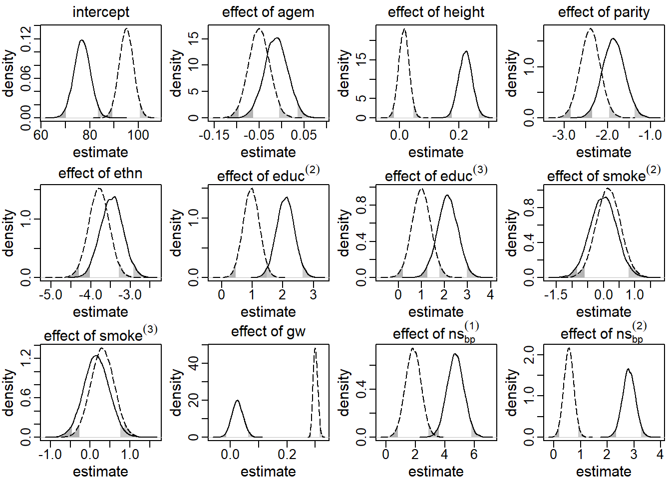
Figure 5.2: Posterior distributions of the main regression coefficients in the first application, derived by the sequential approach. The solid (dashed) line represents the endogenous (exogenous) model. The shaded areas mark values outside the 95% credible interval.
A possible explanation for these differences is that in the exogenous model the
correlation between gw and bp is only captured in the parameter \(\gamma\)
whereas in the endogenous model it is split between \(\gamma\) and the covariance
between the random effects of the model for bp and gw, i.e., the elements in
the upper right quadrant of \(\mathbf D\).
Figure 5.7 in Appendix 5.B.3 shows the posterior
density of these elements of the matrix \(\mathbf D\). Most of the parameters
describing the covariance between \(\mathbf b^\texttt{gw}\) and \(\mathbf b^\texttt{bp}\) estimate the
respective covariance to be different from zero. The exogenous model implies
that these parameters are zero and does not estimate them. Interpreting the
results from the endogenous model we may conclude that gw and bp are
correlated, but that there is no evidence that changes in gw cause changes
in bp.
5.5.2 Association between Gestational Weight Gain and Child BMI
Fetal development follows a well-researched course which is influenced by
maternal health throughout pregnancy. Specifically, the effect of gestational
weight gain may vary between different periods of pregnancy, i.e., different
periods of fetal development. Hence, the effect of trimester-specific weight
gain is often a predictor of interest.
How much weight gain is considered healthy varies with maternal BMI before pregnancy (bmim)
which, therefore, needs to be considered as predictor variable in this research question.
Since gw is observed entirely prior to the outcome (bmi), it might not
be considered to be a time-varying covariate in the narrow sense, i.e., it
does not change throughout the time range of the outcome measurements. Nevertheless,
it does change over time and an appropriate characterization of this change is
essential to obtaining results that allow meaningful conclusions with
regards to the research question at hand.
We calculated trimester specific weight gain as the differences between weight
before pregnancy, 14 weeks of gestation, 27 weeks of gestation and at
(or rather right before) birth (gestbir), and scaled these differences to reflect weight gain
per week. The functional relation between gw and bmi can thus be
represented as
\[
f(H_i^\texttt{gw}(t), t) = \left\{\Delta_1(\texttt{gw}_i), \Delta_2(\texttt{gw}_i),
\Delta_3(\texttt{gw}_i)\right\}^\top,
\]
with
\[\begin{eqnarray*}
\Delta_1(\texttt{gw}_i) &=& \frac{\texttt{gw}_i(\texttt{gage}= 14) - \texttt{gw}_i(\texttt{gage}= 0)}{14},\\
\Delta_2(\texttt{gw}_i) &=& \frac{\texttt{gw}_i(\texttt{gage}= 27) - \texttt{gw}_i(\texttt{gage}= 14)}{27-14},\\
\Delta_3(\texttt{gw}_i) &=& \frac{\texttt{gw}_i(\texttt{gage}= \texttt{gestbir}_i) - \texttt{gw}_i(\texttt{gage}= 27)}
{\texttt{gestbir}_i - 27}.
\end{eqnarray*}\]
As in the first application, we assumed a non-linear evolution of gw over time,
which was modelled using a natural cubic spline for gage with 2 df.
Also, the trajectories of child BMI, for which age and gender-specific standard
deviation scores (SDS) were used, were non-linear and therefore modelled using a
natural cubic spline with 3 df for age, in the formula below represented by
\(\texttt{ns}_i^{(1)}(t)\), \(\texttt{ns}_i^{(2)}(t)\) and \(\texttt{ns}_i^{(3)}(t)\).
Since gw was measured before birth and bmi only after birth, we assumed
that gw was exogenous in this application.
The analysis model for this research question can be written as
\[\begin{eqnarray*}
\texttt{bmi}_i(t) & = & (\beta_0 + b_{i0}^\texttt{bmi}) + \beta_1 \texttt{agem}_i + \beta_2 \texttt{parity}_i
+ \beta_3\texttt{ethn}_i\\
& & + \beta_4\texttt{educ}_i^{(2)} + \beta_5\texttt{educ}_i^{(3)} + \beta_6\texttt{smoke}_i^{(2)}\\
& & + \beta_7\texttt{smoke}_i^{(3)} + \beta_8\texttt{bmim}_i
+ (\beta_{9} + b_{i1}^\texttt{bmi}) \texttt{ns}_i^{(1)}(t)\\
& & + (\beta_{10} + b_{i2}^\texttt{bmi})\texttt{ns}_i^{(2)}(t)
+ (\beta_{11} + b_{i3}^\texttt{bmi})\texttt{ns}_i^{(3)}(t)\\
& & + \gamma_1\Delta_1(\texttt{gw}_i) + \gamma_2\Delta_2(\texttt{gw}_i)
+ \gamma_3\Delta_3(\texttt{gw}_i) + \varepsilon_i^\texttt{bmi}(t),
\end{eqnarray*}\]
The analysis was again performed using the sequential approach, where
imputation models for gw and the baseline covariates were specified
analogous to the first application.
To reduce correlation between the elements of \(\boldsymbol \gamma\), an elastic net
shrinkage hyperprior for the variance parameters of \(\boldsymbol \gamma\) was used
(Mallick and Yi 2013).
Results from the analysis of this second research question are presented in Figure 5.3.
Only the posterior distributions of the parameters relating to bmim
and gw are shown as these are the parameters of interest here.
It can be seen that children of mothers with higher baseline BMI had
higher BMIs as well – an increase of one kg/m2 resulted on average in a
0.03
SDS higher child BMI (95% CI [0.03, 0.04]).
Higher gestational weight gain during the first trimester
was associated with higher child BMI (0.23
SDS increase per kg weekly weight gain; 95% CI
).
Even though the posterior mean of the effect of weekly gestational weight gain
during the second trimester was slightly higher
(0.26),
due to the increased uncertainty of this estimate
(95% CI [-0.08, 0.65])
there was no evidence of an association with the trajectories of child BMI.
There was also no evidence that weight gain during the last trimester was a
relevant predictor of child BMI
(0.12;
95% CI [-0.09, 0.33]).
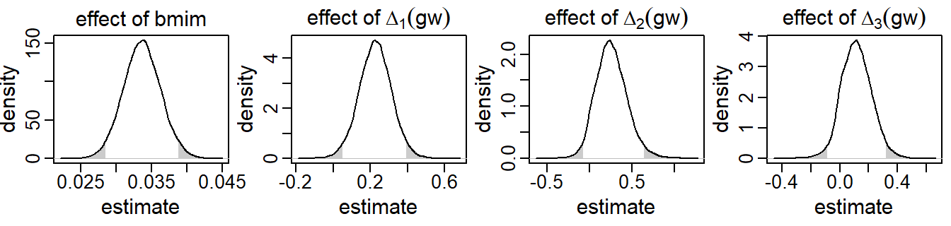
Figure 5.3: Posterior distributions of a selection of regression coefficients from the second application, derived by the sequential approach. The shaded areas mark values outside the 95% credible interval.
5.6 Simulation Study
To evaluate the performance of the two imputation approaches described in Section 5.4 with regards to misspecification of the endo- or exogeneity of a time-varying covariate and the bias introduced by misspecification of the functional form in a more controlled setting, we performed a simulation study in which we compared results from correctly specified models with those that are misspecified, for data generated in a range of different scenarios and different missing mechanisms. Specifically, the key objectives were5.6.1 Design
We simulated 200 datasets in each of six scenarios that differed in the endo-/exogeneity of the covariate, the functional form and the model (sequential or multivariate normal) that was used. Common to all scenarios was that 10 repeated measurements of a normally distributed time-varying covariate and a conditionally normal outcome variable, with measurements at the same, unbalanced time points, were created. Under the sequential approach data was generated with a linear or a quadratic relation between covariate and outcome, where the covariate was either exogenous or endogenous. For the multivariate normal model (which always generates data with a linear relation between the outcome and an endogenous covariate) we considered two scenarios with regards to the correlation of the error terms, where in one scenario the error terms of outcome and covariate were independent and in the other correlated.
Missing values were created in the time-varying covariate according to two MAR mechanisms, in which the probability of the time-varying covariate being missing either only depended on the outcome at the same time point or on the outcome at the same time point as well as the covariate at the previous time point.
Details on the exact setup of the simulation study are given in Appendix 5.C.1.
5.6.2 Analysis Models
Each of the datasets was analysed using both approaches with different assumptions regarding the endo- or exogeneity of the covariate and the functional form, before values were deleted, and for both missing mechanisms.
The complete dataset was analysed using function lmer() from the
R-package lme4 (R Core Team 2016; Bates et al. 2015) as well as with the sequential
approach.
Missing data was imputed and analysed with the sequential approach, where the
random effects were modelled according to the current assumption of exo- or
endogeneity, and the imputation was repeated twice with the multivariate normal
approach (once using the model with independent error terms and once assuming
correlated error terms). Each time, ten imputed datasets were created by drawing
values from the posterior chains of the incomplete covariate and analysed
analogously to the analysis of the complete data.
When the covariate was assumed exogenous, lmer() was used and the
coefficients from the ten corresponding analyses pooled using Rubin’s Rules (Rubin 1987).
When the covariate was assumed to be endogenous, the sequential approach with
correlated random effects was used and the ten sets of posterior MCMC chains
combined to calculate posterior summary measures.
An overview of the assumptions and models used can be found in Table 5.2 in Appendix 5.C.2. The specific parameter values that were used are given in Tables 5.3 and 5.4 in Appendix 5.C.3.
5.6.3 Results
Firstly, we found that the sequential approach provided unbiased estimates when comparing the results from the analysis of the complete data to the true parameters that were used to generate the data. Secondly, in all scenarios, results were very similar for both MAR mechanisms and we will, hence, not distinguish them during the further description of the results.
Regarding to our first objective, the comparison of the sequential and the multivariate normal approach when exo- or endogeneity and functional form were specified correctly, we found that both approaches were unbiased and their 95% credible/confidence intervals had the desired coverage. However, misspecification of the error terms in the multivariate normal approach as independent had the overall largest impact on the results (estimates were on average half the value of the estimate from the analysis of the complete data and CIs had 0% coverage). Based on this finding, we excluded the multivariate normal approach with independent error terms from further comparisons. Moreover, we saw that misspecification of an endogenous covariate as exogenous resulted in bias while misspecification of an exogenous covariate as endogenous did not. This was the case for both approaches, and linear as well as quadratic (only for the sequential approach) functional form. With respect to our third objective, the simulation study showed that imputation with the multivariate normal approach (with correlated error terms) in a setting where the functional form was correctly assumed to be quadratic during the subsequent analysis had the second largest impact, with a relative bias of approximately 0.8, and resulted in CIs with coverage of close to 0%. The bias that was added due to misspecification of the functional form as linear during imputation as well as analysis, as compared to the results from the analysis of the complete data under the same misspecification, was small and overall comparable between the multivariate normal and the sequential approach. These findings were the same irrespective of the exo- or endogeneity of the covariate. Plots of the results from the simulation study as well as a detailed discussion of these results can be found in Appendix 5.C.4.
In summary, the results of this simulation study demonstrate the impact that imprudent acceptance of default assumptions, like exogeneity, linear relations between variables, or (conditioned on random effects) uncorrelated error terms may have.
5.7 Discussion
Motivated by two research questions from the Generation R study, we investigated two Bayesian approaches to handle missing covariate data in models with longitudinal outcomes and time-varying covariates. Specifically, we compared the multivariate normal approach, a widely known omnibus approach, to the more custom-designed sequential approach, which we extended to handle endogenous time-varying covariates. The focus of this comparison was on the ability to take into account different functional relations between such covariates and the outcome, and the suitability for exogenous as well as endogenous covariates.
The analysis of our real data applications illustrated the necessity for methods that allow for complex functional relations and endogenous covariates. Simulation studies confirmed that in our setting, methods that make the common assumption of exogeneity of a time-varying covariate provide biased estimates. The assumption of endogeneity during imputation and analysis, however, did not introduce any bias, which suggests choosing the endogenous specification, e.g., to model the random effects of the outcome and the time-varying covariate correlated, as a default. The simulation study also demonstrated that imputation with the multivariate normal approach in settings where the implied assumption of linear associations between variables is violated can be biased. Furthermore, great care should be taken when assumptions about the correlation structure of the error terms are made in the multivariate normal approach, as misspecification may result in large bias. Results indicated that the sequential approach is more robust with regards to this type of misspecification, however, future research is required to evaluate this further. Overall, the sequential approach performed well and proved to be a suitable method to impute and analyse longitudinal data with possibly endogenous time-varying covariates.
The ability of the sequential approach to handle various functional forms, and to provide estimates in settings with endogenous time-varying covariates, can be seen as its biggest advantages. Moreover, it can handle non-linear associations of baseline covariates and interaction terms involving incomplete covariates without the need of approximations like the “just another variable” approach or passive imputation via transformation (Bartlett et al. 2015; Seaman, Bartlett, and White 2012; White, Royston, and Wood 2011). Even in settings where there is no single functional form of interest, but several candidate functions, it may be applied in combination with shrinkage techniques which may help the decision which functional form is most appropriate.
In the present paper, we focused on a single time-varying covariate and ignorable missing data mechanisms, however, extensions of the sequential approach to accommodate more complex settings are possible. Multiple time-varying covariates can be added to the linear predictor of the analysis model. Imputation models for the time-varying covariates could either be specified assuming conditional independence between different time-varying covariates, i.e., excluding them from each other’s linear predictor, assuming joint multivariate distributions for their random effects and/or error terms, or by specifying a functional form of one time-varying covariate to be included in the linear predictor of another covariate, analogous to the specification of the analysis model described in Section 5.3. The second option may be a convenient choice if a linear relation between the time-varying covariates is a reasonable assumption. When the missing data mechanism is non-ignorable, this can be taken into account by extending the specification of the joint distribution with terms that either describe the selection mechanism (i.e., the missingness pattern given the data) or specify how the distribution of the data depends on the missingness pattern (Carpenter and Kenward 2013; Van Buuren 2012; Daniels and Hogan 2008).
A reason why the multivariate normal approach may be preferred in practice, is its availability in software packages, as, for instance, the R-package jomo (Quartagno and Carpenter 2016) or REALCOM-impute (Carpenter, Goldstein, and Kenward 2011). Those implementations also provide samplers that can handle restricted covariance matrices. More tailored approaches, like the sequential approach, usually need to be implemented by hand, which, however, can be done in existing Bayesian software packages such as JAGS or WinBUGS in a straightforward way. In Appendix 5.C.5 we give example syntax for both approaches. This syntax can easily be extended to include complete or incomplete baseline covariates (see also the Appendix of Erler et al. (2016)). Additional example syntax can be provided upon request.
When imputing and analysing complex datasets, researchers need to deliberate if standard methods that are easy to apply meet the requirements of the application at hand, specifically if the assumptions of those methods are met. It is our opinion that too often this is not the case and standard approaches are applied even when they are not adequate. Therefore, we plead for the use of methods that are flexible enough to be adapted to the specific characteristics of a problem. In the context of imputation and analysis of longitudinal data with possibly endogenous time-varying covariates, the sequential approach presented here is such an approach.
Appendix
5.A Details on the Implied Exo- or Endogeneity
In this section, we provide details on the implications that the approaches introduced in Section 5.4 have for the exo- or endogeneity of the time-varying covariate \(\mathbf s\). For \(\mathbf s\) to be exogenous, the conditions from Section 5.3.3 need to be fulfilled, i.e.,
\[ \left\{\begin{array}{l} \begin{align*} p(y_i(t), f(H^s_i(t), t) \mid H^y_i(t^-), H^s_i(t^-), \boldsymbol\theta) = & p(y_i(t) \mid f(H^s_i(t), t), H^y_i(t^-), H^s_i(t^-), \boldsymbol\theta_1) \times\\ & p(s_i(t) \mid H^y_i(t^-), H^s_i(t^-), \boldsymbol\theta_2)\\[2ex] p(s_i(t) \mid H^s_i(t^-), H^y_i(t^-), \mathbf x_i, \boldsymbol\theta) = & p(s_i(t) \mid H^s_i(t^-), \mathbf x_i, \boldsymbol\theta) \end{align*} \end{array} \right. \]
with \(\boldsymbol\theta^\top = (\boldsymbol\theta_1^\top, \boldsymbol\theta_2^\top)\) and \(\boldsymbol\theta_1 \perp\!\!\!\perp \boldsymbol\theta_2\), where \(H^y_i(t^-)\) and \(H^s_i(t^-)\) denote the history of \(\mathbf y\) and \(\mathbf s\), respectively, up to, but excluding measurements at time \(t\). To abbreviate the notation, we will drop the index \(i\) in the following sections.
5.A.1 Exogeneity of the Sequential Approach with Independent Random Effects
As can easily be seen, the first condition is fulfilled in the sequential approach with independent random effects, since the joint distribution of \(\mathbf y\) and \(\mathbf s\) is specified as the product of the conditional and the marginal distribution and the parameters of these distributions are usually specified to be a priori independent.
To show that the second condition is fulfilled as well, several steps are necessary. Under the assumption that \(s(t)\) is independent from \(H^s(t^-)\) and \(H^y(t)\) given the random effects we can write
\[\begin{eqnarray} p(s(t)\mid H^s(t^-), H^y(t),\mathbf x, \boldsymbol\theta) &=& \int p(s(t),\mathbf b\mid H^s(t^-), H^y(t),\mathbf x, \boldsymbol\theta) \; d\mathbf b\nonumber\\ &=&\int p(s(t) \mid \mathbf b, H^s(t^-), H^y(t),\mathbf x, \boldsymbol\theta)\\ & &\phantom{\int} p(\mathbf b \mid H^s(t^-), H^y(t),\mathbf x, \boldsymbol\theta)\; d\mathbf b\nonumber\\ &=& \iint p(s(t) \mid \mathbf b^s,\mathbf x, \boldsymbol\theta)\; \nonumber\\ & & \phantom{\iint} p(\mathbf b^s,\mathbf b^y \mid H^s(t^-), H^y(t),\mathbf x, \boldsymbol\theta)\, d\mathbf b^s \, d\mathbf b^y. \tag{5.9} \end{eqnarray}\]
Using Bayes theorem, the conditional distribution of the random effects can be rewritten as
\[\begin{eqnarray} p(\mathbf b^s, \mathbf b^y \mid H^s(t^-), H^y(t), \mathbf x, \boldsymbol\theta)\nonumber\\ = \frac{p(\mathbf b^s, \mathbf b^y, H^s(t^-), H^y(t) \mid \mathbf x, \boldsymbol\theta)} {p(H^s(t^-), H^y(t) \mid \mathbf x, \boldsymbol\theta)}\\ = \frac{p(H^s(t^-), H^y(t) \mid \mathbf b^s, \mathbf b^y, \mathbf x, \boldsymbol\theta)\; p(\mathbf b^s, \mathbf b^y \mid \boldsymbol\theta)} {p(H^s(t^-), H^y(t) \mid \mathbf x, \boldsymbol\theta)}.\tag{5.10} \end{eqnarray}\]
With prior independence of \(\mathbf b^y\) and \(\mathbf b^s\), i.e., \(p(\mathbf b^s,\mathbf b^y\mid \boldsymbol\theta) = p(\mathbf b^s\mid \boldsymbol\theta)\; p(\mathbf b^y\mid \boldsymbol\theta)\), and assuming conditional independence of \(H^s(t^-)\) and \(H^y(t)\) given the random effects, the denominator of (5.10) can be split in two factors, \[\begin{eqnarray} p(H^s(t^-), H^y(t) \mid \mathbf x, \boldsymbol\theta)\!\!\! &=&\!\!\!\iint\! p(H^s(t^-), H^y(t) \mid \mathbf b^y, \mathbf b^s, \mathbf x, \boldsymbol\theta)\, p(\mathbf b^y, \mathbf b^s\mid\boldsymbol\theta) \, d\mathbf b^y d\mathbf b^s\nonumber\\ &=&\!\!\! \int p(H^s(t^-) \mid \mathbf b^s, \mathbf x, \boldsymbol\theta)\, p(\mathbf b^s\mid\boldsymbol\theta)\, d\mathbf b^s\nonumber\\ &&\!\!\! \int p(H^y(t) \mid \mathbf b^y, \mathbf x, \boldsymbol\theta)\, p(\mathbf b^y\mid\boldsymbol\theta) \, d\mathbf b^y\nonumber\\ &=&\!\!\! p(H^s(t^-) \mid \mathbf x, \boldsymbol\theta) \, p(H^y(t) \mid \mathbf x, \boldsymbol\theta). \tag{5.11} \end{eqnarray}\] Substituting (5.10) and (5.11) into (5.9), and recognizing that \[ p(s(t) \mid \mathbf b^s,\mathbf x, \boldsymbol\theta)\; p(H^s(t^-)\mid \mathbf b^s, \mathbf x, \boldsymbol\theta) = p(H^s(t)\mid \mathbf b^s, \mathbf x, \boldsymbol\theta), \] allows us to factorize the integrand from (5.9) so that each factor only depends on either \(\mathbf b^y\) or \(\mathbf b^s\). The two integrals can then be solved separately and (5.9) can be simplified as \[\begin{eqnarray*} p(s(t)\mid H^s(t^-), H^y(t),\mathbf x, \boldsymbol\theta) & = & \frac{\int p(H^s(t)\mid \mathbf b^s, \mathbf x, \boldsymbol\theta) \; p(\mathbf b^s \mid \boldsymbol\theta) \; d\mathbf b^s} {p(H^s(t^-) \mid \mathbf x, \boldsymbol\theta)}\\ & & \frac{\int p(H^y(t) \mid \mathbf b^y, \mathbf x, \boldsymbol\theta) \; p(\mathbf b^y\mid \boldsymbol\theta) \; d\mathbf b^y} {p(H^y(t) \mid \mathbf x, \boldsymbol\theta)}\\ & = & \frac{p(H^s(t) \mid \mathbf x, \boldsymbol\theta)}{p(H^s(t^-) \mid \mathbf x, \boldsymbol\theta)}\; \frac{p(H^y(t) \mid \mathbf x, \boldsymbol\theta)}{p(H^y(t) \mid \mathbf x, \boldsymbol\theta)}\\ & = & p(s(t)\mid H^s(t^-),\mathbf x, \boldsymbol\theta)\;\frac{p(H^s(t^-) \mid \mathbf x, \boldsymbol\theta)} {p(H^s(t^-) \mid \mathbf x, \boldsymbol\theta)}\\ & = & p(s(t)\mid H^s(t^-),\mathbf x, \boldsymbol\theta), \end{eqnarray*}\] which shows that for the sequential approach with independent random effects also the second condition for exogeneity is fulfilled.
5.B Analysis of the Generation R Data
5.B.1 Missing Data Patterns
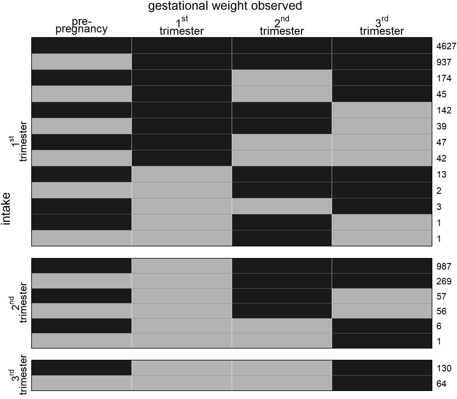
Figure 5.4: Missing data pattern for gestational weight. Dark color depicts observed values, light color missing values. The frequency of each missing data pattern is given on the right.
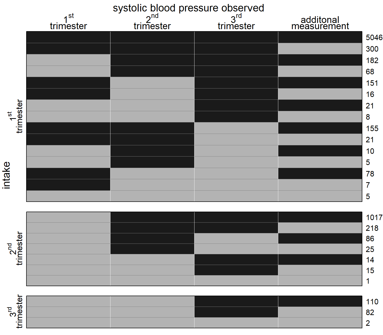
Figure 5.5: Missing data pattern for systolic blood pressure. Dark color depicts observed values, light color missing values. The frequency of each missing data pattern is given on the right.
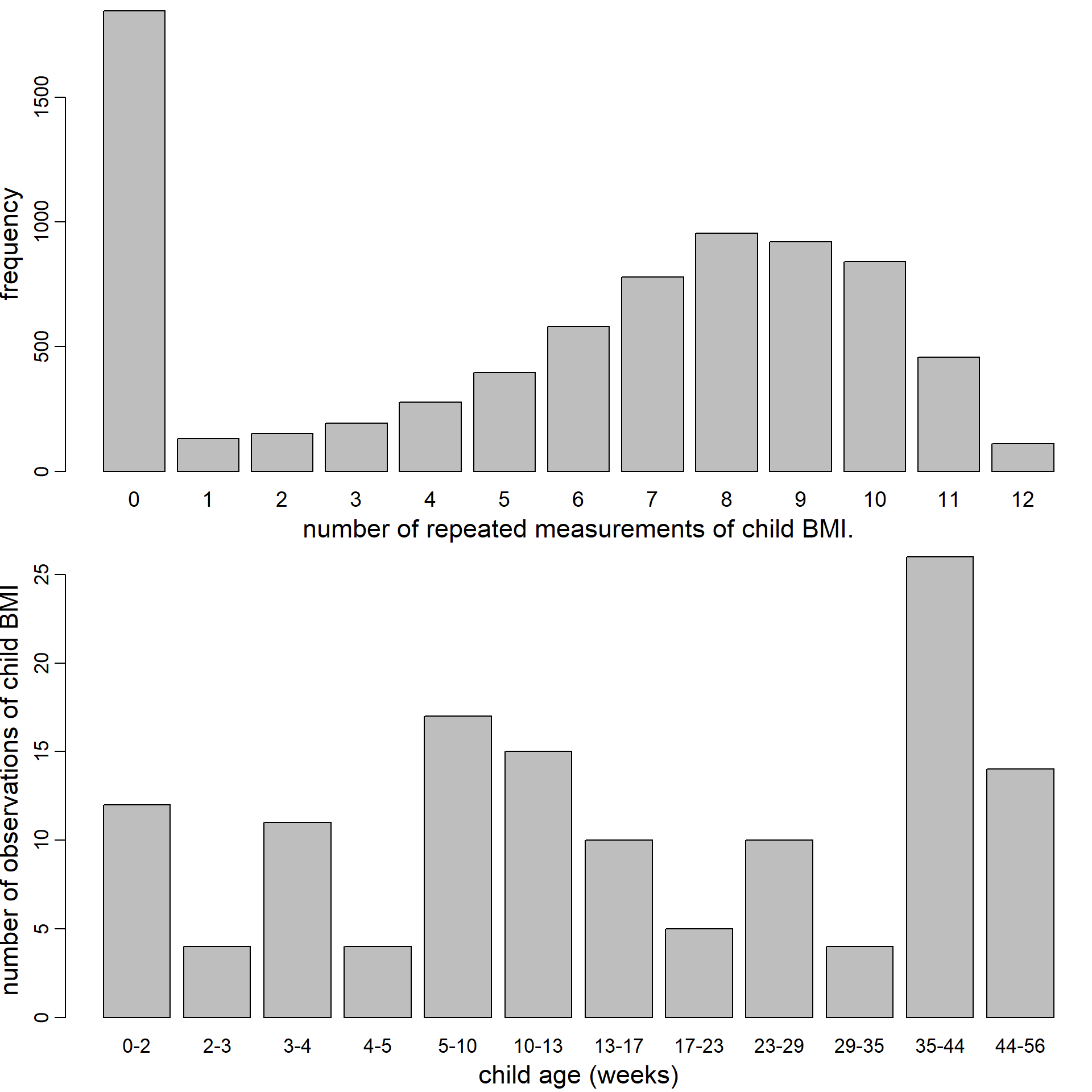
Figure 5.6: Distribution of the number of repeated BMI measurements per child (top) and number of observed values of child BMI per age category (bottom).
5.B.2 Prior Distributions
\[\begin{eqnarray*} \beta_k, \gamma &\overset{iid}{\sim}& N(0, 1000),\qquad k = 0,\ldots, 10\\ \sigma_\texttt{bp}^2, \sigma_\texttt{gw}^2 &\overset{iid}{\sim} & \text{inv-Gamma}(0.01, 0.01)\\ \alpha_k &\sim& N(0, 1000), \qquad k = 0,\ldots, 10\\ \mathbf D_\texttt{bp}&\sim& \text{inv-Wishart}(R_\texttt{bp}, 3)\\ \mathbf D_\texttt{gw}&\sim& \text{inv-Wishart}(R_\texttt{gw}, 3)\\ (\text{diag}(R_\texttt{bp})^\top, \text{diag}(R_\texttt{gw})^\top) & \overset{iid}{\sim}& \text{Gamma}(1, 0.001) \end{eqnarray*}\]
5.B.3 Additional Graphics
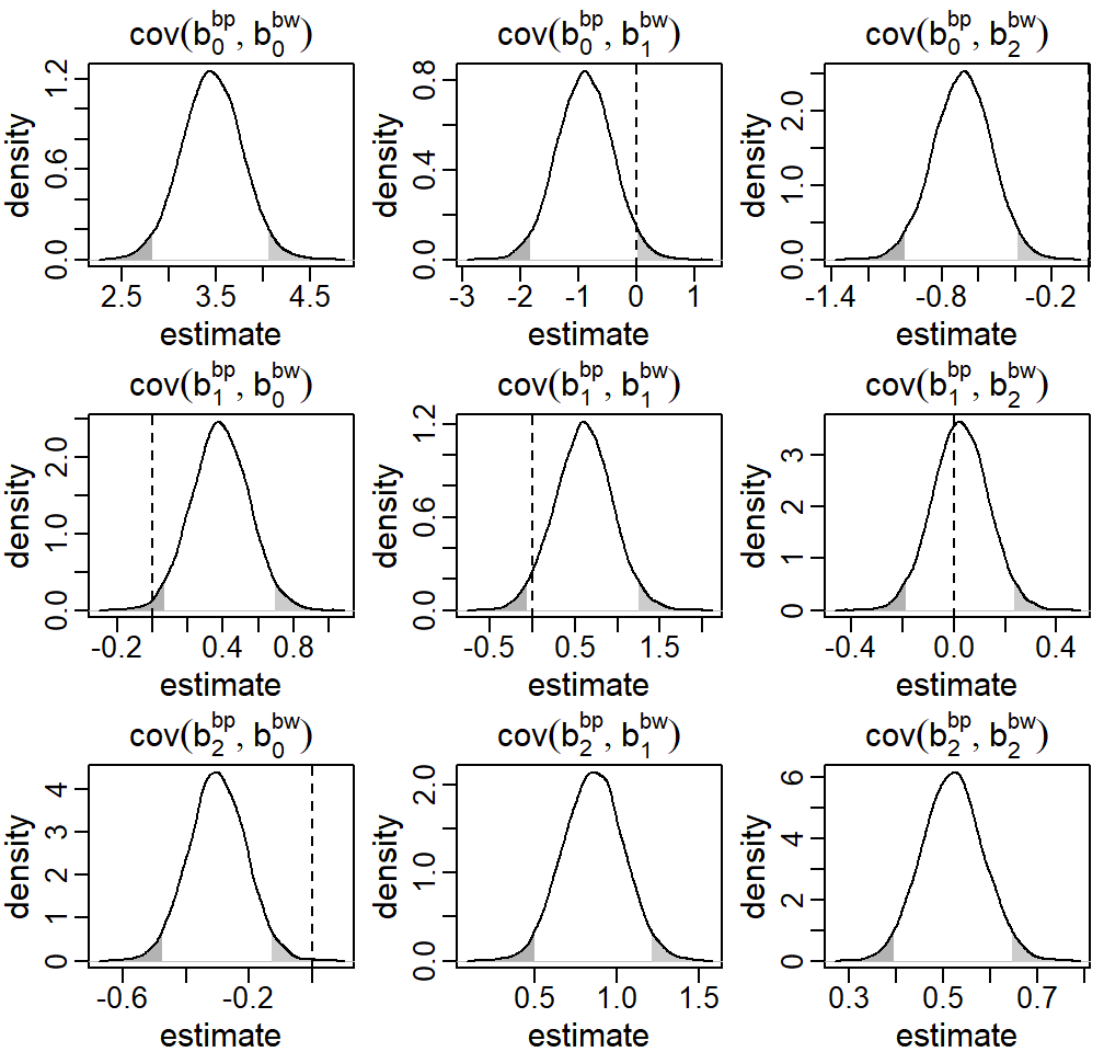
Figure 5.7: Posterior distributions of the covariance between the random effects \(b^\texttt{bp}\) and \(b^\texttt{gw}\) from the endogenous setting in the first motivating question from the Generation R data presented in Section . The dashed vertical line marks zero, i.e., the implied covariance in the exogenous setting, the shaded areas mark values outside the 95% credible interval.
5.C Simulation Study
To evaluate the performance of the two imputation approaches described in Section 5.4 with regards to misspecification of the endo- or exogeneity of a time-varying covariate and the bias introduced by misspecification of the functional form in a more controlled setting, we performed a simulation study in which we compared results from correctly specified models with those that are misspecified, for data generated in a range of different scenarios and different missing mechanisms.
The simulation study was set up to
- confirm that both approaches provide unbiased estimates when the models are correctly specified during imputation and analysis,
- investigate how misspecification of the endo- or exogeneity influences the results, and
- to explore bias due to misspecification of the functional form,
specifically
- the bias introduced during imputation due to the implied linearity assumption of the multivariate normal approach when the true functional form is non-linear, and
- the bias introduced when the imputation model, as well as the analysis model, are misspecified as linear.
5.C.1 Design
We simulated 200 datasets in each of six scenarios that differed in the endo-/exogeneity of the covariate, the functional form and the model (sequential or multivariate normal) that was used. Common in all scenarios was that ten repeated measurements of a normally distributed time-varying covariate and a (conditionally) normal outcome variable, with measurements at the same, unbalanced time points, were created. Table 5.1 gives an overview of the different simulation scenarios. Under the sequential approach data was generated with a linear or a quadratic relation between covariate and outcome, where the covariate was either exogenous or endogenous. The multivariate normal model always generates data with a linear relation between the outcome and an endogenous covariate, however, there we considered two scenarios with regards to the correlation of the error terms, where in one scenario the error terms of outcome and covariate were independent and in the other correlated.
| linear relation | quadratic relation | |
|---|---|---|
| exogenous |
sequential approach seq. (exo., lin.) |
sequential approach seq. (exo., qdr.) |
| endogenous |
sequential approach seq. (endo., lin.) |
sequential approach seq. (endo., qdr.) |
multivariate normal approach
|
The general model used for simulation from the sequential approach was \[\begin{eqnarray} y_{ij} &=& (\beta_{y0} + b_{i0}^y) + (\beta_{y1} + b_{i1}^y) t_{ij} + \boldsymbol\gamma f(s_{ij}) + \varepsilon_{ij}^y \tag{5.12}\\ s_{ij} &=& (\beta_{s0} + b_{i0}^s) + (\beta_{s1} + b_{i1}^s) t_{ij} + \varepsilon_{ij}^s \nonumber \end{eqnarray}\] with \[\begin{eqnarray*} \varepsilon_{ij}^y &\sim& N(0, \sigma_y^2)\\ \varepsilon_{ij}^s &\sim& N(0, \sigma_s^2) \end{eqnarray*}\] and \[\begin{equation*} \left[ \begin{array}{cc} (b_{i0}^y, b_{i1}^y)^\top\\ (b_{i0}^s, b_{i1}^s)^\top \end{array}\right] \sim N\left(\mathbf 0, \left[\begin{array}{cc} \mathbf D_y & \mathbf D_{y,s}\\ \mathbf D_{y,s} & \mathbf D_s \end{array}\right]\right), \end{equation*}\] where \(t_{ij}\) is from a uniform distribution on the interval \([0, 5]\). The specific values of all parameters can be found in Table 5.3 in Appendix 5.C.3. The general model to simulate from a multivariate normal distribution was \[\begin{eqnarray} y_{ij} &=& (\tilde \beta_{y0} + \tilde b_{i0}^y) + (\tilde\beta_{y1} + \tilde b_{i1}^y) t_{ij} + \tilde\varepsilon_{ij}^y \tag{5.13}\\ s_{ij} &=& (\tilde \beta_{s0} + \tilde b_{i0}^s) + (\tilde\beta_{s1} + \tilde b_{i1}^s) t_{ij} + \tilde\varepsilon_{ij}^s\nonumber \end{eqnarray}\] with \[\begin{equation*} \left[ \begin{array}{cc} \tilde\varepsilon_{ij}^y\\ \tilde\varepsilon_{ij}^s \end{array}\right] \sim N \left(\mathbf 0, \left[\begin{array}{cc} \tilde\sigma_y^2 & \tilde\sigma_{y,s}\\ \tilde\sigma_{y,s} & \tilde\sigma_s^2 \end{array}\right]\right) \end{equation*}\]
and \[\begin{equation*} \left[ \begin{array}{c} (\tilde b_{i0}^y, \tilde b_{i1}^y)^\top\\ (\tilde b_{i0}^s, \tilde b_{i1}^s)^\top \end{array}\right] \sim N\left(\mathbf 0, \left[\begin{array}{cc} \mathbf{\widetilde D}_y & \mathbf{\widetilde D}_{y,s}\\ \mathbf{\widetilde D}_{y,s} & \mathbf{\widetilde D}_s \end{array}\right]\right). \end{equation*}\]
With these models, the six different data scenarios were specified as
- seq (exo., lin.):
simulation from model (5.12),
with \(\boldsymbol\gamma f(s_{ij}) = \gamma_1 s_{ij}\) and \(\mathbf D_{y,s} = \mathbf 0\), - seq. (exo., qdr.):
simulation from model (5.12),
with \(\boldsymbol\gamma f(s_{ij}) = \gamma_1 s_{ij} + \gamma_2 s_{ij}^2\) and \(\mathbf D_{y,s} = \mathbf 0\), - seq (endo., lin.): simulation from model (5.12), with \(\boldsymbol\gamma f(s_{ij}) = \gamma_1 s_{ij}\) and \(\mathbf D_{y,s} \neq 0\),
- seq (endo., qdr.): simulation from model (5.12), with \(\boldsymbol\gamma f(s_{ij}) = \gamma_1 s_{ij} + \gamma_2 s_{ij}^2\) and \(\mathbf D_{y,s} \neq 0\),
- mvn (indep. err.): simulation from model (5.13), with \(\mathbf{\widetilde D}_{y,s} \neq \mathbf 0\) and \(\tilde \sigma_{y,s}^2 = 0\),
- mvn (corr. err.): simulation from model (5.13), with \(\mathbf{\widetilde D}_{y,s} \neq \mathbf 0\) and \(\tilde \sigma_{y,s}^2 \neq 0\).
Missing values were created in \(\mathbf s\) according to two MAR mechanisms. In missingness scenario MAR.1, the probability of \(s_{ij}\) being missing depended on \(y_{ij}\) only, while in missingness scenario MAR.2 this probability depended on \(y_{ij}\) as well as \(s_{ij-1}\), specifically \[\begin{align*} \textit{MAR.1:} \qquad \Pr(s_{ij} = \text{NA}) & = \text{expit}(y_{ij} + \zeta_1), \\ \textit{MAR.2:} \qquad \Pr(s_{ij} = \text{NA}) & = \text{expit}(y_{ij} + \zeta_1 + \zeta_2 \unicode{x1D7D9}\;\,(s_{ij-1}<\zeta_3)), \end{align*}\]
where \(\text{expit}(x) = \exp(x)/(1+\exp(x))\) and \(\unicode{x1D7D9}\;\) is the indicator function which is one if the statement is true and zero otherwise. The values for the parameters \(\zeta\) were chosen so that approximately 40% of \(\mathbf s\) were missing and can be found in Table 5.4 in Appendix 5.C.3.
5.C.2 Analysis Models
Each of the datasets was analysed using both approaches with different
assumptions regarding the endo- or exogeneity of the covariate and the
functional form, before values were deleted, and for both missing mechanisms.
An overview of the analysis methods used under the assumptions of either exo-
or endogeneity is given in Table 5.2.
The complete data was analysed using function lmer() from the
R-package lme4 (R Core Team 2016; Bates et al. 2015) as well as with the sequential
approach with independent random effects, \(\mathbf D_{y,s} = \mathbf0\),
when the covariate was assumed to be exogenous, and with the sequential
approach with correlated random effects, i.e., \(\mathbf D_{y,s} \neq \mathbf0\),
when it was assumed to be endogenous. The functional form was specified to be
either linear or quadratic, depending on the current assumption.
Incomplete data from both missing mechanisms was imputed and analysed with the
sequential approach, again with either independent or correlated random effects.
The imputation was repeated with the multivariate normal approach, using the
model with independent error terms as well as the model with correlated error
terms, and imputed datasets were created by drawing two values that were at
least 50 iterations apart from each of the posterior chains of the incomplete
covariate. The resulting ten imputed datasets were analysed analogously to the
analysis of the complete data.
When lmer() was used, the coefficients from the ten corresponding
analyses were pooled using Rubin’s Rules (Rubin 1987) and when the
sequential approach was used, the ten sets of posterior Markov chains were
combined to calculate posterior summary measures.
| assumption | compl. data | MAR.1 & MAR.2 |
|---|---|---|
| exogenous | sequential | sequential |
lmer()
|
multivariate normal (indep. err.) + lmer()
|
|
multivariate normal (corr. err.) + lmer()
|
||
| endogenous | sequential | sequential |
| multivariate normal (indep. err.) + sequential | ||
| multivariate normal (corr. err.) + sequential |
All Bayesian analyses used five parallel MCMC chains and were implemented in JAGS (Plummer 2003), using the R-package rjags (Plummer 2016). Chains were assumed to have converged when the Gelman-Rubin criterion (Gelman, Meng, and Stern 1996) was not more than 1.1 for the parameters of interest, \((\beta_{y0}, \beta_{y1}, \boldsymbol\gamma^\top)\), and not more than 1.25 for other parameters. The number of iterations in the posterior sample necessary to obtain sufficient precision of the posterior estimate was determined based on the sampling error of the chains for \((\beta_{y0}, \beta_{y1}, \boldsymbol\gamma^\top)\), which was required to be less than 5% of the corresponding standard error.
5.C.3 Parameters Values
| sequential model | multivariate normal model |
|---|---|
| coefficients in the model for \(\mathbf y\) | |
| \(\beta_{y0} = -1.00\) | \(\tilde\beta_{y0} = -1.00\) |
| \(\beta_{y1} = 0.80\) | \(\tilde\beta_{y1} = 0.80\) |
| \(\gamma_1 = 1.20\) | |
| \(\gamma_2 = -0.35\) | |
| coefficients in the model for \(\mathbf s\) | |
| \(\beta_{s0} = 2.00\) | \(\tilde\beta_{s0} = 2.00\) |
| \(\beta_{s1} = -0.30\) | \(\tilde\beta_{s1} = -0.30\) |
| (co)variances of the error terms | |
| \(\sigma_y^2 = 0.40\) | \(\tilde\sigma_y^2 = 0.40\) |
| \(\sigma_s^2 = 0.30\) | \(\tilde\sigma_s^2 = 0.30\) |
| \(\tilde\sigma_{y,s} = 0.20\) | |
| (co)variances of the random effects | |
| \(\mathbf{D}_{y} = \left[\begin{array}{rr} 1.413 & 0.166\\ 0.166 & 0.106 \end{array}\right]\) | \(\widetilde{\mathbf{D}}_{y} = \left[\begin{array}{rr} 1.413 & 0.166\\ 0.166 & 0.106 \end{array}\right]\) |
| \(\mathbf{D}_{s} = \left[\begin{array}{rr} 1.500 & -0.202\\ -0.202 & 0.165 \end{array}\right]\) | \(\widetilde{\mathbf{D}}_{s} = \left[\begin{array}{rr} 1.500 & -0.202\\ -0.202 & 0.165 \end{array}\right]\) |
| \(\mathbf{D}_{y,s} = \left[\begin{array}{rr}% 0.022 & -0.015\\% -0.015 & -0.083% \end{array}\right]\) | \(\widetilde{\mathbf{D}}_{y,s} = \left[\begin{array}{rr}% 0.022 & -0.015\\% -0.015 & -0.083% \end{array}\right]\) |
| \(\zeta_1\) | \(\zeta_2\) | \(\zeta_3\) | |
|---|---|---|---|
| seq. (exo., lin.) | -3.20 | -0.5 | 0.0 |
| seq. (endo., lin.) | -3.20 | -0.5 | 0.0 |
| seq. (exo., qdr.) | -1.85 | -0.7 | -0.3 |
| seq. (endo., qdr.) | -1.85 | -0.7 | -0.3 |
| mvn. (indep. err.) | -1.60 | -0.5 | -0.3 |
| mvn. (corr. err.) | -1.60 | -0.5 | -0.3 |
5.C.4 Detailed Discussion of the Results
In this section, we present and discuss the results from the simulation study in detail. We adhere to the list of aims of the simulation study stated above and start with the comparison of the sequential and the multivariate normal approach when exo- or endogeneity and functional form are specified correctly. The relevant part of the results is shown in Figure 5.8 and grouped into four figures, according to whether the data generating model implied an exogenous or endogenous covariate and a linear or quadratic functional relation with the outcome. The six data generating models are indicated by different plotting symbols. The different approaches (sequential and multivariate normal, with independent or correlated error terms) are represented by rows, whereas the columns show three evaluation measures, summarized over all 200 simulated datasets. The relative bias was calculated as the median of the ratios of the estimate (REML estimate or posterior mean) from the analysis of the incomplete data and the estimate from the corresponding complete data analysis, the mean squared error (MSE) as the average of the squared differences between the estimates from the missing and complete data analyses, and the CI-coverage as the proportion of CIs from the missing data analysis that covered the estimate from the corresponding complete data analysis. The desired value for each of these measures is indicated by the vertical line. Since results were similar under both missing mechanisms in most settings and to facilitate readability of the figures, we present results under MAR.1 only. Furthermore, we only present results for the parameter related to the time-varying covariate, \(\boldsymbol \gamma\).
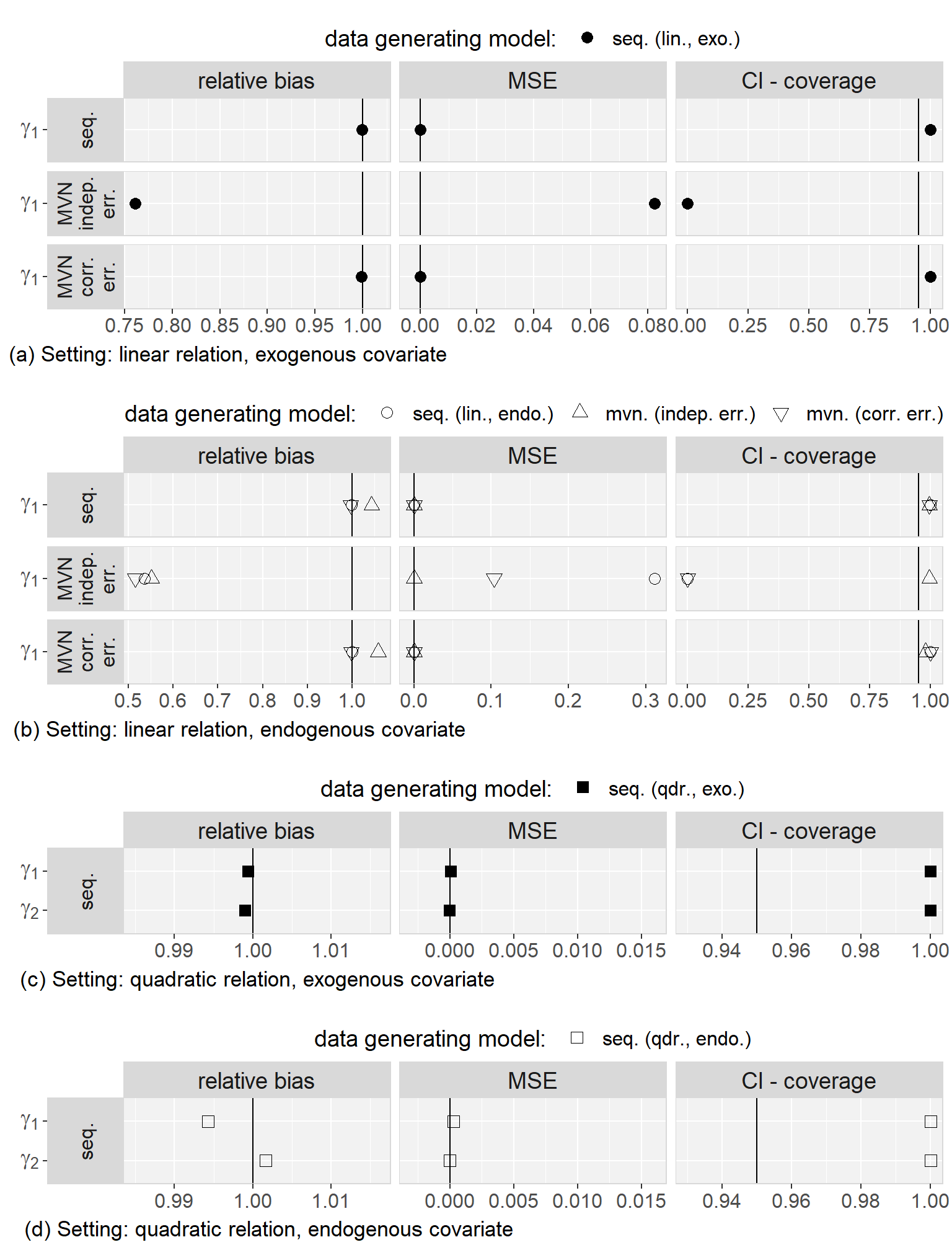
Figure 5.8: Relative bias, mean squared error (MSE), and proportion of CIs that covered the estimate from the analysis of the complete data, when imputation and analysis models were correctly specified with regards to exo- or endogeneity and functional form. The vertical lines mark the respective desired values.
Figure 5.8a shows that the sequential approach as well as the multivariate normal approach with correlated error terms were both unbiased and had CIs that covered the posterior mean from the complete data analysis in all 200 simulations when data was generated with a linear functional form and exogenous covariate. The multivariate normal approach with independent error terms, however, was clearly biased and had CIs that did not cover the estimate from the analysis of the complete data for any of the simulated datasets. It performed even worse in the endogenous setting (shown in Figure 5.8b), unless data was generated by this very model. The multivariate normal approach with correlated error terms and the sequential approach performed well in data that was simulated from the sequential model or the multivariate normal model with correlated error terms, but were biased for data that was generated by the multivariate normal model with independent error terms (relative bias approx. \(1.05\) under MAR.1 and approx. \(1.3\) under MAR.2, for both approaches), however, coverage of the CIs was above 95%.
Corresponding results in the settings with a quadratic relation are shown in Figures 5.8c and 5.8d for the sequential approach, since a correct specification of a quadratic functional form during the imputation procedure is not possible in the multivariate normal approach. Also in these settings, the sequential approach performed well.
The results from the linear setting demonstrate that misspecification of the correlation structure of the error terms may have great impact on the results and we will, therefore, exclude the multivariate normal model with independent error terms in the subsequent comparisons. Note that, since in our simulation \(\varepsilon_{ij}^s\) enters the model for \(y_{ij}\) through \(s_{ij}\), the sequential approach also implies correlation between the error terms.
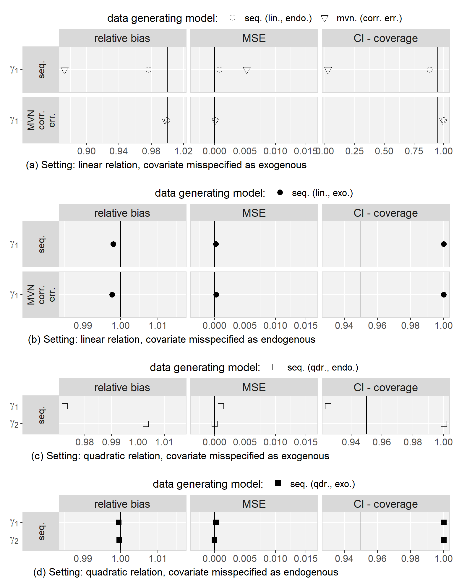
Figure 5.9: Relative bias, mean squared error (MSE), and proportion of CIs that covered the estimate from the analysis of the complete data, when imputation and analysis models were correctly specified with regards to the functional form but misspecified with regards to the exo- or endogeneity of the time-varying covariate. The vertical lines mark the respective desired values.
The second aim of this simulation study was to investigate the effect of misspecification of the exo- or endogeneity during imputation and/or analysis. Figure 5.9 summarizes the relevant results, again split into the different settings with regards to the assumption of exo- or endogeneity and the functional form. The setting in which a linear endogenous covariate is misspecified as exogenous is shown in Figure 5.9a. There, imputation with the multivariate normal approach did not add any bias compared to the (in the same way misspecified) analysis of the complete data, irrespective if the data were generated by the multivariate normal model or the (endogenous) sequential model. Imputation and analysis with the sequential approach with independent random effects introduced some additional bias: for data that was simulated from the sequential approach with correlated random effects, the relative bias was 0.98 and the coverage 88%. When data was simulated from the multivariate normal model, however, the relative bias worsened to 0.87 and the coverage to 2.5%. In the reversed case, where a linear, exogenous covariate was misspecified as endogenous, estimates from both the sequential and the multivariate normal approach were unbiased (see Figure 5.9b). Simulations in the quadratic setting led to corresponding results (for the sequential approach), although the estimates of \(\gamma_2\) were less biased than the estimates of \(\gamma_1\), as can be seen in Figures 5.9c and 5.9d.
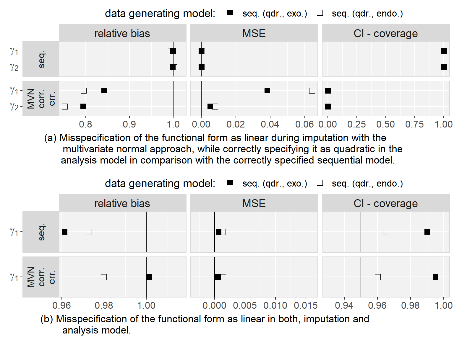
Figure 5.10: Relative bias, mean squared error (MSE), and proportion of CIs that covered the estimate from the analysis of the complete data, when imputation and analysis models were correctly specified with regards to exo- or endogeneity but misspecified with regards to the functional form. The vertical lines mark the respective desired values.
With regards to our third aim, the exploration of bias due to misspecification of the functional form, we investigated two specific issues. First, we explored to what extend misspecification of a quadratic functional form as linear during imputation with the multivariate normal approach, when the functional relation is correctly specified during the subsequent analysis, had an impact on the results. Our findings are summarized in Figure 5.10 and show that this type of misspecification resulted in a relative bias of approximately 0.8 and very bad coverage of the CIs of both parameters, \(\gamma_1\) and \(\gamma_2\), which did not cover the true parameters in any of the simulations.
Second, we extended the misspecification to the analysis model, i.e., assumed that the functional form was linear when the true structure was quadratic. In both approaches, this resulted in only little additional bias compared to the misspecified analysis of the complete data, in the exogenous as well as in the endogenous setting, and had no influence on the coverage of the CIs (see Figure 5.10).
Summarizing the results from our simulation study, we saw that misspecification of the error terms in the multivariate normal approach as independent had the largest impact on the results, leading to estimates that were on average half the value of the estimate from the analysis of the complete data and CIs that had coverage of 0%. For misspecification of an endogenous covariate as exogenous the most severe relative bias that was observed was 0.87 (and a corresponding coverage of the 95% CI of only 2.5%) in the setting where the sequential approach (with independent random effects) was used to impute data that was generated by the multivariate normal model. Imputation with the multivariate normal approach (with correlated error terms) in a setting where the functional form was correctly assumed to be quadratic had the second largest impact, with a relative bias of approximately 0.8, and resulted in CIs that only covered the parameter estimated in the analysis of the complete data in one single simulation for MAR.2. The bias that was added due to misspecification of the functional form as linear during imputation and analysis as compared to the results from the analysis of the complete data under the same misspecification was small (between 0.96 and 1.05) and overall comparable between the multivariate normal and the sequential approach.
5.C.5 JAGS Syntax
We provide here an example of the JAGS (Plummer 2003) syntax that was used in the simulation study. The first part of syntax shows the sequential model assuming \(\mathbf s\) is exogenous and has a linear relation with \(\mathbf y\). We then show how to adapt that syntax for the endogenous setting. The second part contains example syntax that shows how the multivariate normal approach can be implemented in JAGS. There, we present the syntax used in the setting with correlated error terms.
When implementing mixed models in JAGS, it is convenient to use hierarchical centring. This means that the fixed effects enter the linear predictor through the random effects, i.e., the random effects are not centred around zero but around the fixed effects. The syntax differs from the formulas provided in the previous sections to this regard. Note also that normal distributions have to be specified using the precision instead of the variance when using JAGS.
Data / Notation:
TN: number of observations in the datasetN: number of individualspriorR: \(4\times 4\) diagonal matrix of NA values
Sequential Approach
model {
  for (j in 1:TN) {
    # linear mixed effects models for y and s
    y[j] ~ dnorm(mu.y[j], tau.y)
    s[j] ~ dnorm(mu.s[j], tau.s)

    # linear predictors
    # (hierarchical centring specification for baseline effects)
    mu.y[j] <- inprod(b[subj[j], 1:2], Z[j, ]) + beta[3] * s[j]
    mu.s[j] <- inprod(b[subj[j], 3:4], Z[j, ])
  }

  # priors for the precision of y and s
  tau.y ~ dgamma(0.01, 0.01)
  tau.s ~ dgamma(0.01, 0.01)


  # specification of the random effects
  for (i in 1:N) {
    # random effects in the model for y
    b[i, 1:2] ~ dmnorm(mu.b[i, 1:2], inv.D.y[ , ])
    mu.b[i, 1] <- beta[1] # random intercept
    mu.b[i, 2] <- beta[2] # random slope

    # random effects in the model for s
    b[i, 3:4] ~ dmnorm(mu.b[i, 3:4], inv.D.s[ , ])
    mu.b[i, 3] <- alpha[1] # random intercept
    mu.b[i, 4] <- alpha[2] # random slope
  }

  # priors for the fixed effects
  for (k in 1:3) {
    beta[k] ~ dnorm(0, 0.001)
  }
  for (k in 1:2) {
    alpha[k] ~ dnorm(0, 0.001)
  }


  # priors for the precision of the random effects
  for (k in 1:4) {
    priorR[k, k] ~ dgamma(0.1, 0.01)
  }

  # precision and covariance matrix of the random effects
  # in the model for y
  inv.D.y[1:2, 1:2] ~ dwish(priorR[1:2, 1:2], 2)
  D.y[1:2, 1:2] <- inverse(inv.D.y[ , ])

  # precision and covariance matrix of the random effects
  # in the model for s
  inv.D.s[1:2, 1:2] ~ dwish(priorR[3:4, 3:4], 2)
  D.s[1:2, 1:2] <- inverse(inv.D.s[ , ])
}
In the endogenous setting, the specification of the random effects and related priors changes to:
  # specification of the random effects
  for (i in 1:N) {
    b[i, 1:4] ~ dmnorm(mu.b[i, 1:4], inv.D[ , ])

    # random effects in the model for y
    mu.b[i, 1] <- beta[1]
    mu.b[i, 2] <- beta[2]

    # random effects in the model for s
    mu.b[i, 3] <- alpha[1]
    mu.b[i, 4] <- alpha[2]
  }

  # priors for the precision of the random effects
  for(k in 1:4){
    priorR[k, k] ~ dgamma(0.1, 0.01)
  }

  # precision and covariance matrix of the random effects
  inv.D[1:4, 1:4] ~ dwish(priorR[1:4, 1:4], 4)
  D[1:4, 1:4] <- inverse(inv.D[ , ])
}
Multivariate Normal Approach
A natural specification for the distribution of \(\boldsymbol y\) and \(\mathbf s\) in the setting with correlated random effects would be to specify \(\left\{y(t), s(t)\right\}^\top\) as multivariate normal. However, JAGS cannot sample from a multivariate normal distribution when only one component is missing. We therefore have to specify separate univariate normal distributions for \(y(t)\) and \(s(t)\) and additionally a multivariate normal distribution for the error terms \(\left\{\varepsilon_i^y(t), \varepsilon_i^s(t)\right\}^\top\). The precision in the univariate normal distributions for \(y(t)\) and \(s(t)\) is then set to a large value to ``force’’ the variation to be modelled in the multivariate normal distribution of the error terms rather than the two univariate normal distributions.
Data / Notation:
mu.eps= c(0, 0)tau= 10000
model {
  for (j in 1:TN) {
    # linear mixed effects models for y and s
    y[j] ~ dnorm(mu.y[j], tau)
    s[j] ~ dnorm(mu.s[j], tau)

    # linear predictors
    # (hierarchical centring specification and "epsilon trick")
    mu.y[j] <- inprod(b[subj[j], 1:2], Z.y[j, ]) + eps[j, 1]
    mu.s[j] <- inprod(b[subj[j], 3:4], Z.s[j, ]) + eps[j, 2]

    eps[j, 1:2] ~ dmnorm(mu.eps[], inv.Sig[ , ])
  }

  # priors for the precision of y and s
  for (k in 1:2) {
    priorR.invSig[k, k] ~ dgamma(0.1, 0.01)
  }
  inv.Sig[1:2, 1:2] ~ dwish(priorR.invSig[1:2, 1:2], 2)
  Sig[1:2, 1:2] <- inverse(inv.Sig[ , ])


  # specification of the random effects
  for (i in 1:N) {
    # random effects in the model for y
    b[i, 1:4] ~ dmnorm(mu.b[i, 1:4], inv.D[ , ])
    mu.b[i, 1] <- beta[1, 1]
    mu.b[i, 2] <- beta[2, 1]

    # random effects in the model for s
    mu.b[i, 3] <- beta[1, 2]
    mu.b[i, 4] <- beta[2, 2]
  }


  # priors for the precision of the random effects
  for (k in 1:4) {
    priorR.invD[k, k] ~ dgamma(0.1, 0.01)
  }

  # precision and covariance matrix of the random effects
  inv.D[1:4, 1:4] ~ dwish(priorR.invD[1:4, 1:4], 4)
  D[1:4, 1:4] <- inverse(inv.D[ , ])

  # priors for the fixed effects
  for (k in 1:2) {
    beta[k, 1] ~ dnorm(0, 0.001)
    beta[k, 2] ~ dnorm(0, 0.001)
  }
}
References
Andrinopoulou, Eleni-Rosalina, and Dimitris Rizopoulos. 2016. “Bayesian Shrinkage Approach for a Joint Model of Longitudinal and Survival Outcomes Assuming Different Association Structures.” Statistics in Medicin 35 (26): 4813–23. https://doi.org/10.1002/sim.7027.
Bartlett, Jonathan W., Shaun R. Seaman, Ian R. White, and James R. Carpenter. 2015. “Multiple Imputation of Covariates by Fully Conditional Specification: Accommodating the Substantive Model.” Statistical Methods in Medical Research 24 (4): 462–87. https://doi.org/10.1177/0962280214521348.
Bates, Douglas, Martin Mächler, Ben Bolker, and Steve Walker. 2015. “Fitting Linear Mixed-Effects Models Using lme4.” Journal of Statistical Software 67 (1): 1–48. https://doi.org/10.18637/jss.v067.i01.
Carpenter, James R., Harvey Goldstein, and Michael G. Kenward. 2011. “REALCOM-IMPUTE Software for Multilevel Multiple Imputation with Mixed Response Types.” Journal of Statistical Software 45 (1): 1–14. https://doi.org/10.18637/jss.v045.i05.
Carpenter, James R., and Michael G. Kenward. 2013. Multiple Imputation and Its Application. John Wiley & Sons, Ltd. https://doi.org/10.1002/9781119942283.
Daniels, Michael J., and Joseph W. Hogan. 2008. Missing Data in Longitudinal Studies: Strategies for Bayesian Modeling and Sensitivity Analysis. Boca Raton, FL: Chapman & Hall/CRC. https://doi.org/10.1201/9781420011180.
Diggle, Peter, Patrick Heagerty, Kung-Yee Liang, and Scott Zeger. 2002. Analysis of Longitudinal Data. Oxford, United Kingdom: Oxford University Press.
Engle, Robert F., David F. Hendry, and Jean-Francois Richard. 1983. “Exogeneity.” Econometrica 51 (2): 277–304. https://doi.org/10.2307/1911990.
Erler, Nicole S., Dimitris Rizopoulos, Joost van Rosmalen, Vincent W. V. Jaddoe, Oscar H. Franco, and Emmanuel M. E. H. Lesaffre. 2016. “Dealing with Missing Covariates in Epidemiologic Studies: A Comparison Between Multiple Imputation and a Full Bayesian Approach.” Statistics in Medicine 35 (17): 2955–74. https://doi.org/10.1002/sim.6944.
Garrett, Elizabeth S., and Scott L. Zeger. 2000. “Latent Class Model Diagnosis.” Biometrics 56 (4): 1055–67. https://doi.org/10.1111/j.0006-341X.2000.01055.x.
Gelman, Andrew, Xiao-Li Meng, and Hal Stern. 1996. “Posterior Predictive Assessment of Model Fitness via Realized Discrepancies.” Statistica Sinica 6 (4): 733–60.
Ibrahim, Joseph G., Ming-Hui Chen, and Stuart R. Lipsitz. 2002. “Bayesian Methods for Generalized Linear Models with Covariates Missing at Random.” Canadian Journal of Statistics 30 (1): 55–78. https://doi.org/10.2307/3315865.
Kooijman, Marjolein N., Claudia J. Kruithof, Cornelia M. van Duijn, Liesbeth Duijts, Oscar H. Franco, Marinus H. van IJzendoorn, Johan C. de Jongste, et al. 2016. “The Generation R Study: Design and Cohort Update 2017.” European Journal of Epidemiology 31 (12): 1243–64. https://doi.org/10.1007/s10654-016-0224-9.
Lesaffre, Emmanuel M. E. H., and Andrew B. Lawson. 2012. Bayesian Biostatistics. John Wiley & Sons. https://doi.org/10.1002/9781119942412.
Little, Roderick J. A., and Donald B. Rubin. 2002. Statistical Analysis with Missing Data. Hoboken, New Jersey: John Wiley & Sons, Inc. https://doi.org/10.1002/9781119013563.
Lunn, David J., Andrew Thomas, Nicky Best, and David Spiegelhalter. 2000. “WinBUGS – a Bayesian modelling framework: Concepts, structure, and extensibility.” Statistics and Computing 10 (4): 325–37. https://doi.org/10.1023/A:1008929526011.
Mallick, Himel, and Nengjun Yi. 2013. “Bayesian Methods for High Dimensional Linear Models.” Journal of Biometrics & Biostatistics 4 (S3): S1–005. https://doi.org/10.4172/2155-6180.S1-005.
Plummer, M. 2003. “JAGS: A Program for Analysis of Bayesian Graphical Models Using Gibbs Sampling.” Edited by Kurt Hornik, Friedrich Leisch, and Achim Zeileis.
Plummer, Martyn. 2016. rjags: Bayesian Graphical Models using MCMC. https://CRAN.R-project.org/package=rjags.
Quartagno, Matteo, and James R. 2016. jomo: A Package for Multilevel Joint Modelling Multiple Imputation. http://CRAN.R-project.org/package=jomo.
R Core Team. 2016. R: A Language and Environment for Statistical Computing. Vienna, Austria: R Foundation for Statistical Computing. http://www.R-project.org/.
Rubin, Donald B. 1987. Multiple Imputation for Nonresponse in Surveys. Wiley Series in Probability and Statistics. Wiley. https://doi.org/10.1002/9780470316696.
Seaman, Shaun R., Jonathan W. Bartlett, and Ian R. White. 2012. “Multiple Imputation of Missing Covariates with Non-Linear Effects and Interactions: An Evaluation of Statistical Methods.” BMC Medical Research Methodology 12 (1): 46. https://doi.org/10.1186/1471-2288-12-46.
Tielemans, Myrte J., Nicole S. Erler, Elisabeth T. M. Leermakers, Marion van den Broek, Vincent W. V. Jaddoe, Eric A. P. Steegers, Jessica C. Kiefte-de Jong, and Oscar H. Franco. 2015. “A Priori and a Posteriori Dietary Patterns During Pregnancy and Gestational Weight Gain: The Generation R Study.” Nutrients 7 (11): 9383–99. https://doi.org/10.3390/nu7115476.
Van Buuren, Stef. 2012. Flexible Imputation of Missing Data. Chapman & Hall/CRC Interdisciplinary Statistics. Taylor & Francis.
White, Ian R., Patrick Royston, and Angela M. Wood. 2011. “Multiple imputation using chained equations: Issues and guidance for practice.” Statistics in Medicine 30 (4): 377–99. https://doi.org/10.1002/sim.4067.