Bayesian Imputation of Missing Covariates
2019-08-21
Chapter 1 General Introduction
It can be assumed that missing values exist since we started to collect data. The need to find ways to deal with them emerged as the amount of data that was collected grew, but the willingness to provide information to the parties collecting it (often the government for the purpose of the census) abated. The inefficiency due to the loss of information resulting from only using the complete cases for analysis was no longer considered acceptable (Scheuren 2005).
The methods that were used to handle missing values in the 50s and 60s replaced the missing values by a single value, such as ``hot-deck’’ imputation, where a missing value is replaced by an observed value of a case that is similar to the case with the missing value with regards to other, observed characteristics (Andridge and Little 2010; Behrmann 1954; Nordbotten 1963; Gorinson 1969). The idea of replacing a missing datum with multiple values (and arguably the beginning of the development of more sophisticated missing data methods) traces back to Donald B. Rubin, who first described his idea in 1977 (Rubin 2004). He states that
“[…] of course (1) imputing one value for missing datum can’t be correct in general, and (2) in order to insert sensible values for a missing datum we must rely more or less on some model relating unobserved values to observed values.”
The Bayesian framework naturally lends itself to missing data settings, treating missing values as unobserved random variables that have a distribution which depends on the observed data (Rubin 1978a, 1978b). Nevertheless, initially it was not used in these settings since calculations can quickly become very involved when parts of the data are unobserved, and the computational procedures nowadays used to overcome these difficulties were not yet available. In this thesis, we focus on inference on missing data under the Bayesian paradigm but compare it to other, commonly used approaches.
1.1 Mechanisms and Patterns of Missing Data
1.1.1 Missing Data Mechanism
In the context of missing data, strictly speaking, the term “data” does not only refer to the values of those variables that were intended to be measured, but also includes the missing data indicator, a binary variable, that describes if a value was observed or not.
Using this missingness indicator, a model for the missing data mechanism can be postulated. This model describes how the probability of a value being missing is related to other characteristics of the same unit. It can be written as \[p(\mathbf R\mid \mathbf X_{obs}, \mathbf X_{mis}, \boldsymbol\psi),\] where \(\mathbf R\) is the missing data indicator matrix and \(\mathbf X_{obs}\) and \(\mathbf X_{mis}\) denote the part of the data that is completely observed and the part of the data that has missing values for some subjects, respectively.
In general, the model for the missing data mechanism must be taken into account when analysing incomplete data, however, under certain conditions, it may be ignored. Conditions for ignorability were introduced by Rubin (1976) and are closely connected to the well-established classification of missing data mechanisms described below (Little and Rubin 2002).
Missing Completely at Random
The data is said to be missing completely at random (MCAR) when the probability of a value being missing does not depend on any data, that is, when \(p(\mathbf R\mid \mathbf X_{obs}, \mathbf X_{mis}, \boldsymbol\psi) = p(\mathbf R\mid \boldsymbol\psi)\). This type of missingness may occur when samples are lost, participants miss a visit or do not fill in a question in a questionnaire, because of reasons that are unrelated with the study for which the data was supposed to be collected.
Missing at Random
In settings in which the probability of a value being missing does depend on factors associated with the study, but those factors have been observed, i.e., are part of \(\mathbf X_{obs}\), the missing data mechanism is called missing at random (MAR) and can be formally described as \(p(\mathbf R\mid \mathbf X_{obs}, \mathbf X_{mis},\boldsymbol\psi) = p(\mathbf R\mid \mathbf X_{obs},\boldsymbol\psi)\). Missing values of this type may occur for instance when in a survey about the consumption of sweets overweight participants are less likely to respond to the question how much chocolate they eat, and the weight of all participants is known. Another example is a longitudinal study where subjects are excluded from future measurements once a critical value is exceeded. MAR includes MCAR as a special case.
Missing Not at Random
When the assumption of MAR does not hold, and the probability of a value being missing does depend on unobserved data, which may either be the missing value itself, unobserved values of other variables, or variables that have not been recorded at all, the missing data mechanism is called missing not at random (MNAR) and can be written as \(p(\mathbf R\mid \mathbf X_{obs}, \mathbf X_{mis},\boldsymbol\psi) \neq p(\mathbf R\mid \mathbf X_{obs},\boldsymbol\psi).\) Examples for data missing not at random would be if, in the above survey, participants who are overweight are more likely not to report their weight, or, if in the longitudinal study the value that exceeded the threshold would not be recorded. Since \(\mathbf X_{mis}\) is not observed, it is not possible to test whether the assumption of MAR holds. Good knowledge of how the data was obtained and why values are missing is necessary to make appropriate assumptions about the missing data mechanism.
Ignorability
In settings where the missing data mechanism is MAR and the parameters of the missingness model, \(\boldsymbol\psi\), are a priori independent / distinct of the parameters of the data model, \(\boldsymbol\theta\), i.e., \(p(\boldsymbol\psi, \boldsymbol\theta) = p(\boldsymbol\psi) \; p(\boldsymbol\theta)\), the missingness process does not need to be explicitly modelled when Bayesian or likelihood inference for \(\boldsymbol\theta\) is performed. Then, the missingness is called ignorable. Throughout this thesis, we assume that this is the case.
1.1.2 Missing Data Pattern
When values are missing in multiple variables, different patterns of missingness can arise. If variables can be ordered such that if a value is missing, the values of all variables following in the sequence are also always missing, the missing data pattern is called monotone (left panel of Figure 1.1). If such an order does not exist, the missing data pattern is non-monotone (right panel of Figure 1.1).
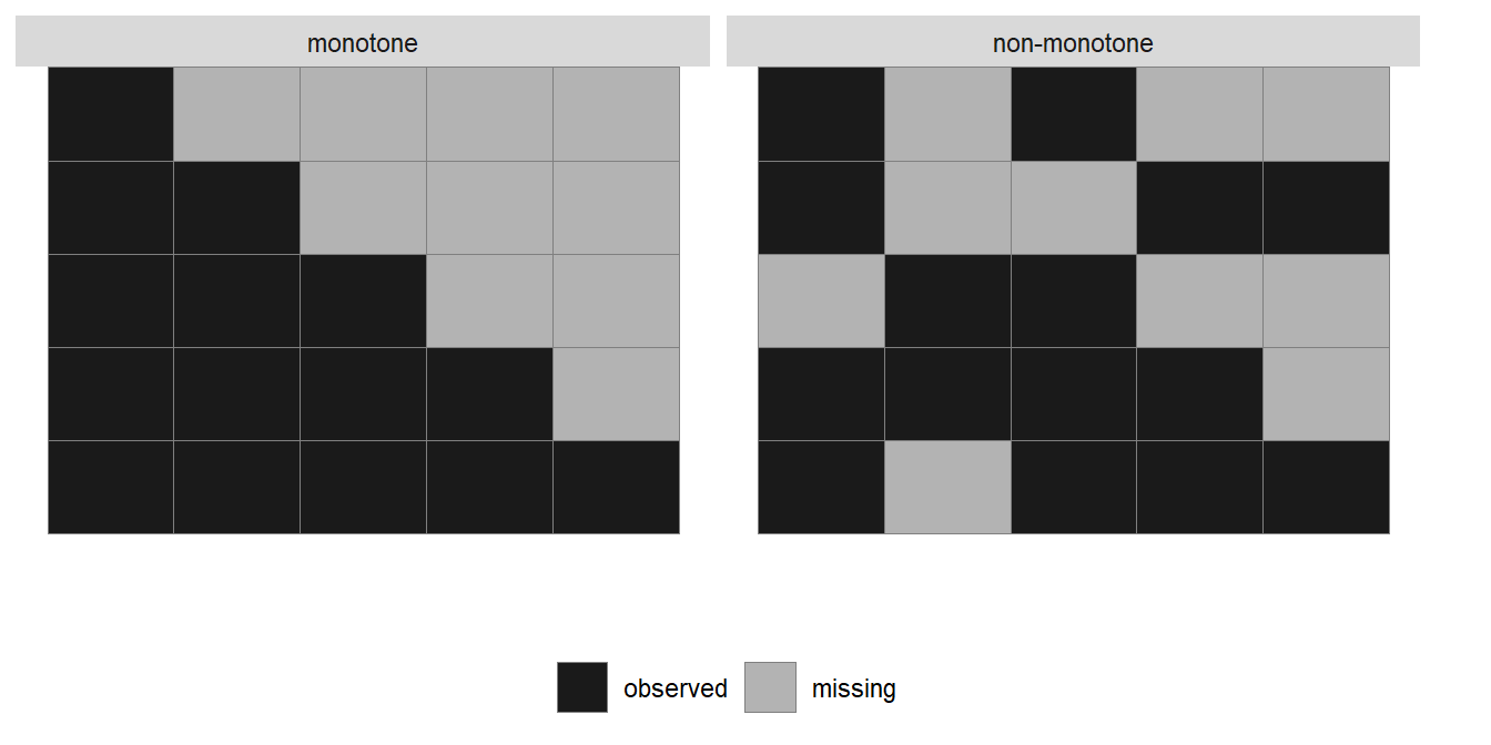
Figure 1.1: Visualization of a monotone and a non-monotone missing data pattern. Each column represents a variable, while rows represent different patterns of missing values.
Monotone missing data patterns typically arise in longitudinal studies with drop-out, where once a patient has left the study, no further measurements are available. In studies where multiple variables measuring different aspects are obtained, either at the same time point or over time, non-monotone missing data patterns occur more frequently, since study participants do not return a particular questionnaire or miss a single visit to the research centre. In this thesis, we consider general, non-monotone missing data patterns.
1.2 Multiple Imputed Datasets
When the concept of multiple imputation was developed in the 1970s, a requirement for a practical way to deal with missing data was that it allowed many researchers to analyse the incomplete data. Moreover, it was essential that these analyses could be done using only standard techniques and software tools, which required complete, balanced data, and without the need of in-depth knowledge of missing data methods (Scheuren 2005). Especially the second part of this requirement is still relevant today since analyses are often performed by researchers without expert knowledge in statistics, who are usually only familiar with standard complete data methods and are not versed in Bayesian methodology.
Rubin’s solution to this practicality issue was to perform imputation once and to distribute the imputed data to various researchers. In this imputation procedure, multiply imputed, i.e., completed, versions of the original data were produced, which differed only in the values that had been filled in for the missing observations. This allowed retaining some information on the uncertainty about the missing values, while each of the datasets could be analysed using standard methods. Since the imputed datasets are not identical, the estimates obtained from the analysis of each dataset will vary. This variation in the obtained estimates allows assessing the additional uncertainty in the effect estimates that is caused by the missing values (Rubin 2004).
In the following, we first give an overview of some popular (Bayesian and non-Bayesian) methods that have been proposed for creating imputed values and then describe the most commonly used procedure to pool the results from the analyses of multiple imputed datasets.
1.2.1 Methods for Imputation
The task to create the imputed values requires to sample from the (posterior) predictive distribution of the unobserved data, given the observed data. Especially in larger datasets, with missing values in multiple variables, possibly of different measurement levels, and a non-monotone missing data pattern, this distribution is multivariate and not of any standard form.
Joint Model Imputation
Rubin’s suggestion in his initial paper on multiple imputation from 1977 (Rubin 2004) was to approximate the posterior predictive distribution with a multivariate normal distribution if variables are continuous, or with a multinomial distribution if data is categorical. Since sampling from either of these distributions is fast and readily available in software, this approach, especially using the multivariate normal distribution, is still used today (Carpenter and Kenward 2013). To allow for covariates of mixed type, the assumption is made that categorical variables have an underlying normal distribution and that different categories are observed depending on the value of that latent distribution. Due to its ability to impute incomplete baseline as well as time-varying covariates in multi-levels settings, we apply and investigate this approach in Chapter 5 of this thesis.
Expectation Maximization
A general approach that allows performing likelihood inference when parts of the data are unobserved, is the Expectation Maximization (EM) algorithm, introduced by Dempster, Laird, and Rubin (1977). The algorithm alternates between the expectation (E) step, in which the expected value of missing data, conditional on observed data and current estimates of the parameters, is obtained, and the maximisation (M) step, in which parameter values are estimated by maximizing the likelihood of the parameters given the current values of the missing data. Even though the approach was not specifically developed to create multiple imputations, it could be applied in this way, if, once the algorithm has converged, not the expectation of missing values is determined, but instead multiple values are drawn from the estimated distribution. In settings where incomplete variables have non-linear associations with other variables, however, the distribution in the M-step may not have a closed form and updating the parameters becomes difficult.
Data Augmentation
Data augmentation, an approach similar to the EM algorithm, was proposed by Tanner and Wong (1987). It can be thought of as a Bayesian version of the EM algorithm since it has the same two-step structure, but the E step is replaced by imputation of missing values and the M step by estimation of the posterior distribution instead of maximization of the likelihood. The motivation behind augmenting the data is that sampling from \(p(\boldsymbol\theta \mid \mathbf X)\) is often easier than sampling from \(p(\boldsymbol\theta \mid \mathbf X_{obs})\) and works well if sampling of \(p(\mathbf X_{mis}\mid \mathbf X_{obs}, \boldsymbol\theta)\) is possible. Nonetheless, even when Monte Carlo integration is used, sampling from distributions that are not members of the exponential family may be difficult, diminishing the attractiveness of the approach. While Tanner and Wong (1987) aimed to estimate the posterior distribution, Li (1988) focused on imputing values but used essentially the same algorithm.
The approach for analysis of incomplete data and imputation of missing values followed throughout this thesis uses data augmentation in conjunction with the Gibbs sampler. The joint distribution of all data, observed and unobserved, as well as the parameters, is specified in a sequence of univariate distributions. Using Gibbs sampling, missing values are imputed by draws from the full conditional distributions arising from this joint distribution. Once the observed data is augmented by the imputed values, posterior inference for the parameters of interest can be obtained as if the data had been complete. The approach is described in detail in Chapter 2.
Multiple Imputation using Chained Equations
The nowadays most popular approach for creating multiple imputations, introduced by Van Buuren, Boshuizen, and Knook (1999), also uses the idea of the Gibbs sampler but is a (mostly) frequentist approach. In multiple imputation using chained equations (MICE), also called multiple imputation using a fully conditional specification (FCS), a full conditional distribution is specified for each incomplete variable and imputed values are sampled from these distributions. If a multivariate distribution exists that has the specified distributions as its full conditionals, the algorithm is a Gibbs sampler.
Specifying the full conditional distributions directly has the advantage that it allows for a flexible algorithm, in which distributions can be tailored to the measurement level of each variable, and sampling is performed on a variable by variable basis using samplers that are easy to implement. The MICE algorithm (Van Buuren 2012) starts by randomly drawing starting values from the set of observed values. Then, in each iteration \(t = 1, \ldots, T\), it cycles once through all incomplete variables \(\mathbf x_j,\; j = 1,\ldots,p\). For each incomplete variable \(j\), the currently completed data except \(x_j\) is defined as \(\mathbf{\dot X}_{-j}^t = \left(\mathbf{\dot x}_1^t, \ldots, \mathbf{\dot x}_{j-1}^t, \mathbf{\dot x}_{j+1}^{t-1}, \ldots, \mathbf{\dot x}_p^{t-1}\right).\) The parameters of the model for \(\mathbf x_j\), \(\boldsymbol{\dot\theta}_j^t\), are sampled from their distribution conditional on the observed part of \(\mathbf x_j\) and the currently completed data of the other variables from subjects that have \(\mathbf x_j\) observed: \[p(\boldsymbol\theta_j^t \mid \mathbf{x}_j^{obs}, \mathbf{\dot X}_{-j}, \mathbf R).\] Imputed values \(\mathbf{\dot x}_j^t\) are drawn from the predictive distribution of the missing values \(\mathbf{x}_{j}^{mis}\) given the other variables and parameters \(\boldsymbol{\dot\theta}_j^t\), \[p(\mathbf x_j^{mis}\mid \mathbf X_{-j}^t, \mathbf R, \boldsymbol \theta_j^t).\] By filling in the imputed values of the last iteration, i.e., \(\left(\mathbf{\dot x}_1^\top, \ldots, \mathbf{\dot x}_p^\top\right)\) into the original, incomplete, data, one imputed dataset is created. The algorithm is run multiple times with different starting values to create a set of multiply imputed datasets.
A drawback of the MICE algorithm is that there is no guarantee that a joint distribution exists that has the specified conditional distributions as its full conditionals. If no such distribution exists, the algorithm may not converge to the correct distribution. Despite this theoretical limitation, it has been shown to work well in practice as long as the conditional distributions fit the data well enough (Zhu and Raghunathan 2015). In settings where incomplete covariates are involved in non-linear functional forms or interactions, or with complex outcomes, such as survival or longitudinal outcomes, specification of correct imputation models is often not feasible (Bartlett et al. 2015; Carpenter and Kenward 2013). Even specification of models that adequately include all information necessary to obtain valid imputations is not straightforward, and, in practice, often not even attempted when imputation is performed by researchers who are unaware that naive use of imputation software will lead to violation of important assumptions and thereby faulty imputations and biased inference. The performance of MICE when used naively for imputation of covariates in longitudinal data is the topic of Chapter 2 of this thesis.
1.2.2 Pooling Results from Multiple Imputed Datasets
Irrespective of the method used for producing imputations, the results from the analyses of the multiple imputed datasets need to be combined in a manner that takes into account the added uncertainty due to the missing values. The formulas for pooling of such results proposed by Rubin and Schenker (1986) (see also Rubin (1987)), usually referred to as Rubin’s Rules, have gained wide acceptance and are outlined in the following.
For a parameter vector \(\mathbf Q\) the overall estimate, pooled over the analyses of \(m\) imputed datasets, can be calculated as the mean over the estimates from these analyses, \[\mathbf{\overline Q} = \frac{1}{m} \sum_{\ell = 1}^m\mathbf{\widehat Q}_\ell,\] where \(\mathbf{\widehat Q}_\ell\) denotes the estimate obtained from the \(\ell\)-th imputed set. The overall variance of \(\mathbf Q\) consists of the within imputation variances \(\mathbf{\overline W}\), which can be calculated by averaging over the estimated variances of the \(\mathbf Q_\ell\) from each imputed dataset, \(\mathbf{\widehat W}_\ell\), \[\mathbf{\overline W} = \frac{1}{m} \sum_{\ell = 1}^m \mathbf{\widehat W}_\ell,\] and the between imputation variance, \(\mathbf B\), calculated as \[\mathbf B = \frac{1}{m-1}\sum_{\ell = 1}^m \left(\mathbf{\widehat Q}_\ell - \mathbf{\overline Q}\right)\left(\mathbf{\widehat Q}_\ell - \mathbf{\overline Q}\right)^\top.\] Following Rubin and Schenker (1986), the total variance, \(\mathbf T\) is the sum of within and between imputation variance, plus an additional term \(\mathbf B/m\), correcting for the finite number of imputations, i.e., \(\mathbf T = \mathbf{\overline W} + \mathbf B + \mathbf B/m\). The relative increase in variance that is due to the missing values can be estimated as \(r_m = \left(\mathbf B + \mathbf B/m \right) / \mathbf{\overline W}\).
The \((1 - \alpha)\) 100% confidence interval for scalar \(Q\) can be calculated as \(\overline Q \pm t_\nu(\alpha/2)\sqrt{T},\) where \(t_{\nu}\) is the \(\alpha/2\) quantile of the \(t\)-distribution with \(\nu = \left(m - 1\right)\left(1 + r_m^{-1}\right)^2\) degrees of freedom.
The corresponding p-value is the probability \(Pr\{F_{1,\nu} > \left(Q_0-\overline Q\right)^2/T\},\) where \(F_{1,\nu}\) is a random variable that has an F distribution with \(1\) and \(\nu\) degrees of freedom, and \(Q_0\) is the null hypothesis value (typically zero).
In the above calculation, the degrees of freedom \(\nu\) are derived under the assumption that there are infinite degrees of freedom in the complete data, denoted \(\nu_{com}\) (Barnard and Rubin 1999). Since this is not a reasonable assumption for small datasets, Barnard and Rubin (1999) proposed a different calculation of the degrees of freedom for the \(t\)-distribution \[\tilde \nu = \left(\frac{1}{\nu} + \frac{1}{\hat\nu_{obs}}\right)^{-1} = \nu_m\left(1 + \frac{\nu}{\hat\nu_{obs}}\right)^{-1} = \nu_{com}\left[\left\{\lambda(\nu_{com})(1-\hat\gamma_m)\right\}^{-1} + \frac{\nu_{com}}{\nu} \right]\] where the observed-data degrees of freedom, \(\nu_{obs}\), are estimated as \(\hat\nu_{obs} = \lambda(\nu_{com})\nu_{com}(1-\hat\gamma_m)\), \(\hat\gamma_m = r_m/(1+r_m)\) and \(\lambda(\nu) = (\nu + 1)(\nu + 3).\) This small-sample version of Rubin’s Rules is implemented in the R package mice and used in this thesis.
1.3 The Bayesian Framework
Since the focus of this thesis is on inference for missing data under the Bayesian paradigm, in this section we will briefly introduce the Bayesian framework and some relevant concepts.
The idea behind the Bayesian paradigm is that inference about an unknown parameter can be obtained by updating an initial guess or prior belief about that parameter with data (Bayes, Price, and Canton 1763; Laplace 1774).
1.3.1 Bayes Theorem
The posterior distribution, i.e., the distribution of a parameter \(\boldsymbol\theta\) conditional on the data \(\mathbf X\), can be expressed as \[p(\boldsymbol\theta\mid X) = \frac{p(\mathbf X\mid \boldsymbol\theta)\; p(\boldsymbol\theta)}{\int_{-\infty}^\infty p(\mathbf X\mid\boldsymbol\theta)\; p(\boldsymbol\theta)\; d\boldsymbol\theta}.\] In the above equations, \(p(\boldsymbol\theta)\) denotes the prior distribution of \(\boldsymbol\theta\), i.e., the distribution of \(\boldsymbol\theta\) that is assumed without taking into account the collected data, \(p(\mathbf X\mid\boldsymbol\theta)\) is the likelihood of the data given the parameter, and the denominator constitutes the marginal distribution of the data, i.e., the distribution of data under all possible values of \(\boldsymbol\theta\), and is often called the normalizing constant. Since this normalizing constant does not depend on \(\boldsymbol \theta\), Bayes theorem is often simplified to \[p(\boldsymbol \theta\mid \mathbf X) \propto p(\mathbf X\mid \boldsymbol\theta)\; p(\boldsymbol\theta),\] i.e., the posterior distribution is proportional to the product of the likelihood and the prior distribution.
In the Bayesian framework, the distribution relating unobserved values, \(\mathbf X_{mis}\), to observed values, \(\mathbf X_{obs}\), referred to by Rubin in his statement given above, is called the posterior predictive distribution of the missing data given the observed data, \[p(\mathbf X_{mis}\mid \mathbf X_{obs}) = \int p(\mathbf X_{mis}\mid \mathbf X_{obs}, \boldsymbol\theta)\; p(\boldsymbol\theta\mid \mathbf X_{obs}) \; d\boldsymbol\theta.\]
In practice, an analytic calculation of the posterior distribution is often not feasible. In that case, it has to be approximated or determined numerically. A numeric method that is frequently used and works in complex settings is the Monte Carlo method.
1.3.2 Monte Carlo Methods
Instead of determining the posterior distribution analytically, the Monte Carlo method (Metropolis and Ulam 1949) draws random samples from it and uses these samples to calculate summary measures of the distribution, to approximate the corresponding measures of the posterior distribution.
Using the central limit theorem, the precision of this approximation to the sample mean, \(\bar{\theta}\), can be determined as \[\bar{\theta'} \pm 1.96\; \text{sd}(\theta')/\sqrt{K},\] where \(K\) is the number of independently sampled values \(\theta'\), and \(\text{sd}(\theta')/\sqrt{K}\) is called the Monte Carlo error.
In high-dimensional settings, however, even “just” sampling from the posterior distribution may not be feasible, since no sampler is available for direct sampling from a multivariate distribution of unknown form, and factorization of the distribution would require solving multiple integrals (Lesaffre and Lawson 2012). The development of Markov Chain Monte Carlo methods (Metropolis et al. 1953; Hastings 1970) was crucial in overcoming this difficulty.
1.3.3 Markov Chain Monte Carlo
The idea behind Markov Chain Monte Carlo (MCMC) sampling is to construct a Markov chain that has the distribution to be sampled from as its stationary distribution. It is an iterative procedure in which a sequence of random variables is created by repeatedly drawing values from a distribution that depends on the previously drawn value. MCMC methods, hence, perform dependent sampling. By creating a Markov chain that has the posterior distribution as its stationary distribution, samples from that stationary distribution can, thus, be regarded as a sample from the posterior distribution.
1.3.4 Gibbs Sampler
The Gibbs sampler, introduced by Geman and Geman (1984), facilitates sampling from high-dimensional distributions by splitting a multivariate problem into a set of univariate problems. It uses the property that a joint distribution is fully specified by its corresponding set of full conditional distributions. Iteratively sampling from these, often univariate, distributions is usually relatively easy. Using Gibbs sampling to obtain draws in an MCMC chain, hence, allows sampling from high-dimensional posterior distributions.
1.3.5 Convergence, Mixing and Thinning
As previously mentioned, samples from an MCMC chain are only samples from the posterior distribution once the chain has converged, i.e., when the distribution of the values remains stable throughout further iterations. In order to obtain valid inferences, convergence of the chains must be checked, and, if necessary, samples from before the chain has converged need to be discarded. The iterations before the chain has converged are called burn-in period.
Convergence may be checked visually, by plotting the drawn values against the iteration number in a so-called traceplot, which should show a horizontal band with no apparent trends or patterns. In this thesis, we additionally evaluated convergence using a statistical criterion developed by Gelman and Rubin (1992). It uses multiple, independent chains for the same parameter, and compares within and between chain variances. When this criterion, which we refer to as the Gelman-Rubin criterion in the rest of this thesis, is close enough to one, say, no more than 1.2, the MCMC chains can be assumed to have converged.
Another potential issue when working with MCMC methods is that they perform dependent sampling. When this dependence is strong it can take many iterations before the MCMC chain converges and, moreover, many iterations until the chain has sufficiently explored the whole range of the posterior distribution. In order to provide enough information about the posterior distribution, a chain with high auto-correlation may have to be continued for more iterations than can practically be handled. To reduce the number of samples that have to be stored, a chain may be thinned out so that only a reduced number of samples is saved.
1.4 Motivating Datasets
The research presented in this thesis is motivated by several large cohort studies. Such studies are especially prone to missing values since typically a large number of variables are measured, and many variables are self-reported (i.e., by questionnaire) or participants have to visit a research centre for measurements to be taken. Moreover, participants are from the general population and may not always see a direct personal benefit in complying with the study protocol.
Two datasets that were used in this thesis for demonstration of the statistical methods under investigation, as well as the real world application of the proposed approach, are briefly introduced in the following sections.
The Generation R Study
The Generation R Study (Kooijman et al. 2016) is an ongoing longitudinal population-based prospective cohort study from fetal life until young adulthood, investigating growth development and health of children, conducted in Rotterdam, the Netherlands. Approximately 10000 pregnant women from the Rotterdam area with an expected delivery date between 2002 and 2006 were included and are followed up, together with their children, until the offspring is 18 years of age. Data is collected at scheduled visits to the research centre as well as by questionnaire, phone interviews or home visits, and augmented by registry information. Among other things, information on maternal diet and lifestyle, health and complications during pregnancy, child growth and health outcomes (e.g., asthma or infectious diseases), behaviour and cognition, body composition and obesity, and eye and tooth development, is collected at different time points.
The National Health and Nutrition Examination Survey
The National Health and Nutrition Examination Survey (NHANES), conducted by the National Center for Health Statistics in the United States, is a large cohort of children and adults and investigates a broad range of health and nutrition related issues (National Center for Health Statistics (NCHS) 2011). Since 1999, a new cohort of approximately 5000 participants, chosen representatively of the US population, is included every year. Data on demographic, socioeconomic, dietary and health-related topics is obtained by interviews and physiological, dental and medical examinations, and laboratory tests are performed. The study is designed to, among other things, investigate risk factors for and prevalence of diseases, get insights into how nutrition (advice) may be used for disease prevention and to inform public health policies.
1.5 Outline of this Thesis
This section provides a brief overview of the content of the subsequent chapters.
In Chapter 2 a fully Bayesian approach to analysis and imputation of data with incomplete covariate information is described in detail for the setting with a continuous longitudinal outcome and incomplete baseline covariates.
Moreover, different approaches to the handling of a longitudinal outcome in multiple imputation using MICE are investigated, both the naive but commonly used, and other, more sophisticated techniques. MICE and the fully Bayesian approach are compared using a simulation study and a real data example from the Generation R Study, in which the association between maternal diet during pregnancy and gestational weight throughout pregnancy is analysed. This application is motivated by the study conducted in Chapter 3.
Chapters 3 and 4 contain applications of the presented Bayesian approach using data from the Generation R Study. In Chapter 3 the association between guideline-based (a priori) and data-driven (a posteriori) dietary patterns with gestational weight gain and trajectories of gestational weight are investigated. Using the approach presented in Chapter 2, simultaneous analysis of the trajectories of gestational weight and imputation of incomplete baseline covariates is performed. The imputed data is then used in the secondary analysis to investigate the association of diet with weight gain.
Chapter 4 examines the effect of sugar containing beverage consumption by pregnant women on body composition of their offspring. Measures of body composition are the body mass index (BMI), which was measured repeatedly, and the fat mass index and fat-free mass index, both measured when children where approximately six years of age. All three outcomes are modelled jointly, and imputation of incomplete baseline covariates is performed using the Bayesian approach presented in Chapter 2.
In Chapter 5, the approach of Chapter 2 is extended to time-varying covariates. Additional issues that arise with such covariates, specifically the potential endogeneity and non-linear shape of the association with the outcome are considered. Advantages and disadvantages as well as the performance of the proposed approach are compared to multiple imputation using a multivariate normal model in a simulation study and two research questions from the Generation R Study: the association between blood pressure and weight of mothers during pregnancy, and the association of maternal gestational weight and child BMI from birth until five years of age.
The implementation of our fully Bayesian approach to jointly analyse and impute incomplete data into the R package JointAI is described in Chapter 6. Functionality of the package to analyse incomplete data using generalized linear mixed models or generalized linear regression models, which may include non-linear forms or interaction terms, is demonstrated in detail. Data from the NHANES study as well as data simulated to mimic data from a longitudinal cohort study, such as the Generation R Study, is used to illustrate this functionality.
The thesis concludes in Chapter 7 with a general discussion of limitations of the proposed approach which arise from the model assumptions, and propositions as to how the approach and its implementation in software should be further improved and extended to facilitate valid inference with incomplete data in a wider range of applications and settings.
References
Andridge, Rebecca R., and Roderick J. A. Little. 2010. “A Review of Hot Deck Imputation for Survey Non-Response.” International Statistical Review 78 (1): 40–64. https://doi.org/10.1111/j.1751-5823.2010.00103.x.
Barnard, John, and Donald B. Rubin. 1999. “Miscellanea. Small-Sample Degrees of Freedom with Multiple Imputation.” Biometrika 86 (4): 948–55. https://doi.org/10.1093/biomet/86.4.948.
Bartlett, Jonathan W., Shaun R. Seaman, Ian R. White, and James R. Carpenter. 2015. “Multiple Imputation of Covariates by Fully Conditional Specification: Accommodating the Substantive Model.” Statistical Methods in Medical Research 24 (4): 462–87. https://doi.org/10.1177/0962280214521348.
Bayes, Thomas, Richard Price, and John Canton. 1763. “An Essay towards solving a Problem in the Doctrine of Chances.” Philosophical Transactions 53: 370–418. https://doi.org/10.1098/rstl.1763.0053.
Behrmann, Herbert I. 1954. “Sampling Technique in an Economic Survey of Sugar Cane Production.” South African Journal of Economics 22 (3): 326–36. https://doi.org/10.1111/j.1813-6982.1954.tb01646.x.
Carpenter, James R., and Michael G. Kenward. 2013. Multiple Imputation and Its Application. John Wiley & Sons, Ltd. https://doi.org/10.1002/9781119942283.
Dempster, Arthur P., Nan M. Laird, and Donald B. Rubin. 1977. “Maximum likelihood from incomplete data via the EM algorithm.” Journal of the Royal Statistical Society. Series B (Methodological), no. 1: 1–38. http://www.jstor.org/stable/2984875.
Gelman, Andrew, and Donald B. Rubin. 1992. “Inference from Iterative Simulation Using Multiple Sequences.” Statistical Science 7 (4): 457–72. https://doi.org/10.1214/ss/1177011136.
Geman, Stuart, and Donald Geman. 1984. “Stochastic Relaxation, Gibbs Distributions, and the Bayesian Restoration of Images.” IEEE Transactions on Pattern Analysis and Machine Intelligence, no. 6: 721–41. https://doi.org/10.1109/TPAMI.1984.4767596.
Gorinson, Morris. 1969. “How the Census Data Will Be Processed.” Monthly Labor Review (Pre-1986); Washington 92 (12): 42. http://www.jstor.org/stable/41837533.
Hastings, Wilfred K. 1970. “Monte Carlo Sampling Methods Using Markov Chains and Their Applications.” Biometrika 57 (1): 97–109. https://doi.org/doi:10.2307/2334940.
Kooijman, Marjolein N., Claudia J. Kruithof, Cornelia M. van Duijn, Liesbeth Duijts, Oscar H. Franco, Marinus H. van IJzendoorn, Johan C. de Jongste, et al. 2016. “The Generation R Study: Design and Cohort Update 2017.” European Journal of Epidemiology 31 (12): 1243–64. https://doi.org/10.1007/s10654-016-0224-9.
Laplace, Pierre-Simon. 1774. “Mémoire Sur La Probabilité Des Causes Par Les évènemens.” Mémoires de Mathématque et Physique, Presentés à L’Académie Royale Des Sciences, Par Divers Savans & Lûs Dans Ses Assemblées, Tome Sixiéme 66: 621–56.
Lesaffre, Emmanuel M. E. H., and Andrew B. Lawson. 2012. Bayesian Biostatistics. John Wiley & Sons. https://doi.org/10.1002/9781119942412.
Li, Kim-Hung. 1988. “Imputation using Markov chains.” Journal of Statistical Computation and Simulation 30 (1): 57–79.
Little, Roderick J. A., and Donald B. Rubin. 2002. Statistical Analysis with Missing Data. Hoboken, New Jersey: John Wiley & Sons, Inc. https://doi.org/10.1002/9781119013563.
Metropolis, Nicholas, Arianna W. Rosenbluth, Marshall N. Rosenbluth, Augusta H. Teller, and Edward Teller. 1953. “Equation of State Calculations by Fast Computing Machines.” The Journal of Chemical Physics 21 (6): 1087–92. https://doi.org/10.1063/1.1699114.
Metropolis, Nicholas, and Stanislaw Ulam. 1949. “The Monte Carlo Method.” Journal of the American Statistical Association 44 (247): 335–41. https://doi.org/10.2307/2280232.
National Center for Health Statistics (NCHS). 2011. “National Health and Nutrition Examination Survey Data.” U.S. Department of Health and Human Services, Centers for Disease Control and Prevention. https://www.cdc.gov/nchs/nhanes/.
Nordbotten, Svein. 1963. “Automatic Editing of Individual Statistical Observations.” In. Statistical Standards and Studies 3. United Nations Statistical Commission; Economic Commission for Europe. Conference of European Statisticians. http://hdl.handle.net/11250/178265.
Rubin, Donald B. 1976. “Inference and Missing Data.” Biometrika 63 (3): 581–92. https://doi.org/10.2307/2335739.
Rubin, Donald B. 1978a. “Bayesian Inference for Causal Effects: The Role of Randomization.” The Annals of Statistics 6 (1): 34–58. https://doi.org/10.1214/aos/1176344064.
Rubin, Donald B. 1978b. “Multiple Imputations in Sample Surveys - A Phenomenological Bayesian Approach to Nonresponse.” In Proceedings of the Survey Research Methods Section of the American Statistical Association, 1:20–34. American Statistical Association.
Rubin, Donald B. 1987. Multiple Imputation for Nonresponse in Surveys. Wiley Series in Probability and Statistics. Wiley. https://doi.org/10.1002/9780470316696.
Rubin, Donald B. 2004. “The Design of a General and Flexible System for Handling Nonresponse in Sample Surveys.” The American Statistician 58 (4): 298–302. https://doi.org/10.1198/000313004X6355.
Rubin, Donald B., and Nathaniel Schenker. 1986. “Multiple Imputation for Interval Estimation from Simple Random Samples with Ignorable Nonresponse.” Journal of the American Statistical Association 81 (394): 366–74. https://doi.org/10.2307/2289225.
Scheuren, Fritz. 2005. “Multiple Imputation: How It Began and Continues.” The American Statistician 59 (4): 315–19. https://doi.org/10.1198/000313005X74016.
Tanner, Martin A., and Wing Hung Wong. 1987. “The Calculation of Posterior Distributions by Data Augmentation.” Journal of the American Statistical Association 82 (398): 528–40. https://doi.org/10.2307/2289457.
Van Buuren, Stef. 2012. Flexible Imputation of Missing Data. Chapman & Hall/CRC Interdisciplinary Statistics. Taylor & Francis.
Van Buuren, Stef, Hendriek C. Boshuizen, and Dick L. Knook. 1999. “Multiple Imputation of Missing Blood Pressure Covariates in Survival Analysis.” Statistics in Medicine 18 (6): 681–94. https://doi.org/10.1002/(SICI)1097-0258(19990330)18:6<681::AID-SIM71>3.0.CO;2-R.
Zhu, Jian, and Trivellore E. Raghunathan. 2015. “Convergence Properties of a Sequential Regression Multiple Imputation Algorithm.” Journal of the American Statistical Association 110 (511): 1112–24. https://doi.org/10.1080/01621459.2014.948117.